Huggingface 🤗 is all you need for NLP and beyond

Atharva
@kaggle 4x Expert
Natural Language Processing is one of the fastest-growing fields in Deep Learning. NLP has completely changed since the inception of Transformers. Later on, variants of Transformer architecture where-in only the encoder part was used (BERT) cracked the transfer learning game in NLP. Now, you can download a pre-trained model from the internet which is already trained on huge amounts of data and has the knowledge of language and use it for your downstream tasks with a bit of fine-tuning.
If you are into Deep Learning, you might have heard about HuggingFace. They are the pioneers when it comes to NLP. More than 5000 organizations are using HuggingFace today. Hugging Face is now worth $2 billion and recently became a bi-unicorn 🦄🦄. They aim to build the GitHub of Machine Learning and they are rightly marching towards it. Check out the Forbes article here covering the news.
HuggingFace provides a pool of pre-trained models to perform various tasks in NLP, audio, and vision.
Here are the reasons why you should use HuggingFace for all your NLP needs
State-of-the-art models available for almost every use-case
The models are already pre-trained on lots of data, so you can use them directly or with a bit of finetuning, saving an enormous amount of compute and money
Variety of common datasets are available to test your new ideas
Easy to use and consistent APIs
Supports PyTorch, TensorFlow, and JAX
A highly interactive website where you can search with tags and filters
An interactive widget for each model where you can test the model on the website itself
An interactive widget to view the datasets
Great documentation and model/dataset card which provides a high-level overview of it
HuggingFace Spaces - allows you to host your web apps in a few minutes
AutoTrain - allows to automatically train, evaluate and deploy state-of-the-art Machine Learning models
Inference APIs - over 25,000 state-of-the-art models deployed for inference via simple API calls, with up to 100x speedup, and scalability built-in
Amazing community!
There are many more features of HuggingFace, I would suggest exploring them on their website
The main aim of the blog is to:
- Provide an overview of the
datasetslibrary. - Provide an overview of the
Trainerclass. - Highlight some useful features of
Traineranddatasets. - Show how to customise
Trainerfor your specific needs. - Show how to implement custom models while keeping them consistent with the API.
- Show how to write custom callbacks.
- Weights & Biases integration for experiment tracking.
Some things to keep in mind while reading the blog post 👇
HuggingFace is referred as 🤗 in further part of blog post.
Many words have clickable links. I would suggest visiting them as they provide more information about the topic.
HuggingFace Datasets Library
🤗 Datasets is a library for easily accessing and sharing datasets, and evaluation metrics for Natural Language Processing (NLP), computer vision, and audio tasks.
🤗 datasets allow you to load datasets using a single line of code, use powerful preprocessing methods and quickly get your dataset ready for training in a deep learning model. 🤗 datasets are memory-mapped using Apache Arrow and cached locally. This means that only the necessary data will be loaded into memory, allowing the possibility to work with a dataset that is larger than the system memory (e.g. c4 is hundreds of GB, mc4 is several TB). 🤗 datasets can work on local files, data in memory (e.g. a pandas data frame or a dict), or easily pull from over 1,500 datasets from the Hugging Face Hub. For the large datasets, a streaming mode is also possible, so that you don't have to download a ton of data. Many functions mirror their analogs in sklearn or pandas, and you can even stick the dataset straight into a PyTorch DataLoader.
At the time of writing this post, there are currently over 2568 datasets available on HuggingFace Hub. You can also take an in-depth look inside a dataset with the live Datasets Viewer.
🤗 datasets support a wide range of methods for loading, pre-processing, caching data, etc. Since it's not possible to cover each of them in this blog post, I would recommend this great notebook by Nicholas Broad where he demonstrates a lot of useful methods in 🤗 datasets. Also, their documentation and tutorials are well explained and you can just go through them. They have also explained the technical concepts behind the API.
HuggingFace Trainer Class
The 🤗 Trainer class provides an API for feature-complete training in PyTorch for most standard use cases. This eliminates the need to re-writing the PyTorch training loop from scratch every time you work on a new problem and reduces a lot of boiler-plate code allowing you to focus on the problem at hand and not on engineering aspects of Deep Learning.
If you have experience in writing PyTorch training loops from scratch then you might agree that it becomes a complete mess after adding some custom features like mixed-precision, gradient accumulation with a bunch of if-else statements. This makes the code hard to maintain and increases the possibility of making mistakes in the implementation, which might not get noticed quickly because Deep Learning code is the home of silent bugs.
🤗 Trainer aims to solve this problem by providing an API that can be used for almost all standard use-cases. However, if you want to inject some custom behaviours for a specific use case, you can always do that by overriding that particular method. You can also add callbacks to do certain things while keeping your main training/evaluation loop clean.
Before we dive into the core of this blog, here I've listed out some features of Trainer:
- Automatic checkpointing based on a particular metric
- Mixed Precision
- Gradient Accumulation
- Gradient Clipping
- Gradient Checkpointing
- Custom metric calculation after each evaluation phase
- Multi-GPU training (with just a change of flag/argument)
- TPU training (with just a change of flag/argument)
- Auto find batch size (automatically finds the maximum batch size that can be fit into the GPU's memory)
- Dynamic Padding and Uniform Length Batching (reduces training time significantly)
- Automatic experiment tracking (Supported platforms are azure_ml, comet_ml, mlflow, tensorboard, and wandb)
- push models to the hub (push your trained model to HuggingFace Hub and share it with the community)
- And much more!
In this blog post, I would take the data from an ongoing Kaggle competition. The reason for taking a completely new dataset and not the standard ones like IMDB is to show how to use and customise datasets and Trainer for fairly new and complicated problems. By the end of this blog post, you would get a complete idea of 🤗 datasets and 🤗 Trainer and you would be able to use them for almost all of your NLP problems.
Let's get started ...
About the problem
The dataset is from an ongoing Kaggle competition, U.S. Patent Phrase to Phrase Matching. In this competition, we have to identify similar phrases in U.S. Patents. You can read about the problem statement in detail from the overview page.
In short, we will train our models on a novel semantic similarity dataset to extract relevant information by matching key phrases in patent documents. Determining the semantic similarity between phrases is critically important during the patent search and examination process to determine if an invention has been described before.
Setup
Before we dive into the problem, let's do some initial setups. First, we will install the 🤗 datasets, 🤗 transformers, and Weights & Biases libraries and then download the data. You can download the data from the data tab of the competition.
Note: From here on this will be a code-heavy blog post. Make sure you grab a cup of coffee ☕️ and fire up a Jupyter notebook (either locally if you have a GPU or on colab/kaggle). You can also use spot instances of jarvislabs.ai which provides RTX 5000 at just $0.19/hr and is great for quick experimentations. For this blog post, I am using jarvislabs.ai's RTX 5000 spot instance.
You can fire up your spot instance by creating an account, adding some credits, and toggling the Reserved button to No.
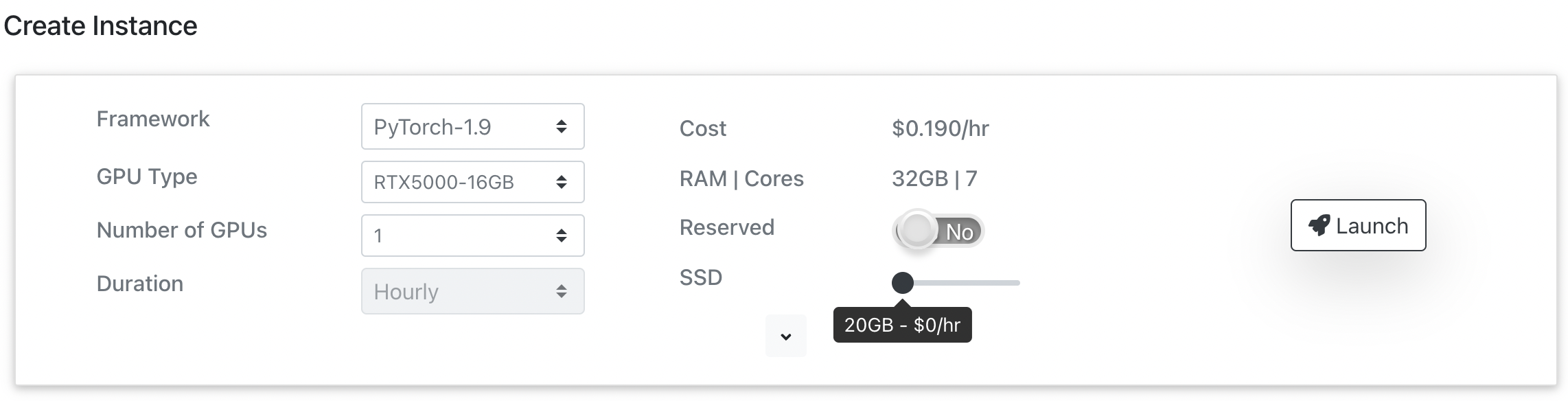
Your instance would be ready within 30 seconds after you click launch and you would get options to connect via SSH, JupyterLab, or VSCode. You can use the JupyterLab and VSCode interface in your browser itself. For this blog post, we will use JupyterLab. Click on the green-colored play button and it will redirect you to a JupyterLab instance.

After your instance is setup, you can sanity check what GPU you are working on.
!nvidia-smi --query-gpu=gpu_name --format=csv

# execute !nvidia-smi to get complete information about the GPU (VRAM, CUDA version, etc)
Output:
    name
    Quadro RTX 5000
# install necessary libraries
!pip install -q datasets transformers sentencepiece wandb
Read Data
Once the essential libraries are installed, we are ready to load the data. Make sure you have downloaded the data from the data page of the competition and placed it in appropriate folder.
import os

# change the `BASE_DIR` to your data's root directory
BASE_DIR = "/home/input"

train_csv_path = os.path.join(BASE_DIR, "train.csv")
test_csv_path = os.path.join(BASE_DIR, "test.csv")
You can load the dataset which is in csv format using 🤗 datasets library. They provide a lot of options to load and manipulate the data and the data is always convertible to other formats seamlessly.
The load_dataset method provides various ways to load and split the data. As our dataset is in csv format we will pass csv in the load_dataset method and path of the file.
from datasets import load_dataset

dataset = load_dataset("csv", data_files=train_csv_path)
dataset
Output:
    Using custom data configuration default-e7c8a3b069ccf5f4


    Downloading and preparing dataset csv/default to /home/.cache/huggingface/datasets/csv/default-e7c8a3b069ccf5f4/0.0.0/433e0ccc46f9880962cc2b12065189766fbb2bee57a221866138fb9203c83519...

    Dataset csv downloaded and prepared to /home/.cache/huggingface/datasets/csv/default-e7c8a3b069ccf5f4/0.0.0/433e0ccc46f9880962cc2b12065189766fbb2bee57a221866138fb9203c83519. Subsequent calls will reuse this data.

    DatasetDict({
        train: Dataset({
            features: ['id', 'anchor', 'target', 'context', 'score'],
            num_rows: 36473
        })
    })
As you can see from the output above, the dataset is already cached which allows for faster loading in further iterations. DatasetDict is a dict object with train, validation, and test as keys and datasets as values. We have only provided train data in the above code cell, that's why we only have train as a key.
But what if we want a validation set as well to validate our experiments? Well, we can do that using load_dataset's split argument. Generally, in Kaggle competitions validation data is not provided separately. We have to generate it from the train data using a leak-free validation strategy because the score on validation data is the only score we can trust throughout the competition to avoid overfitting to the public leaderboard and prevent shake-ups.
There are several ways to split a dataset in 🤗 datasets, below I have demonstrated a few of them which are most commonly used. The first one is to split the data by percentage. You can pass the percentage slice you want in the split argument.
train[:80%] tells that give me the first 80 percent of the data. train[80%:] tells that give me the data after the first 80 percent of data (i.e. last 20% of data).
Note that, this is similar to the slicing we do in python.
train_dataset = load_dataset("csv", data_files=train_csv_path, split="train[:80%]")
valid_dataset = load_dataset("csv", data_files=train_csv_path, split="train[80%:]")
Output:
    Using custom data configuration default-e7c8a3b069ccf5f4
    Reusing dataset csv (/home/.cache/huggingface/datasets/csv/default-e7c8a3b069ccf5f4/0.0.0/433e0ccc46f9880962cc2b12065189766fbb2bee57a221866138fb9203c83519)
    Using custom data configuration default-e7c8a3b069ccf5f4
    Reusing dataset csv (/home/.cache/huggingface/datasets/csv/default-e7c8a3b069ccf5f4/0.0.0/433e0ccc46f9880962cc2b12065189766fbb2bee57a221866138fb9203c83519)
train_dataset, valid_dataset
Output:
    (Dataset({
         features: ['id', 'anchor', 'target', 'context', 'score'],
         num_rows: 29178
     }),
     Dataset({
         features: ['id', 'anchor', 'target', 'context', 'score'],
         num_rows: 7295
     }))
We can also split the data after loading in sklearn syntax style as shown below
dataset = load_dataset("csv", data_files=train_csv_path, split="train")

splits = dataset.train_test_split(test_size=0.2, seed=2022)  # sklearn syntax
splits
Output:
    Using custom data configuration default-e7c8a3b069ccf5f4
    Reusing dataset csv (/home/.cache/huggingface/datasets/csv/default-e7c8a3b069ccf5f4/0.0.0/433e0ccc46f9880962cc2b12065189766fbb2bee57a221866138fb9203c83519)

    DatasetDict({
        train: Dataset({
            features: ['id', 'anchor', 'target', 'context', 'score'],
            num_rows: 29178
        })
        test: Dataset({
            features: ['id', 'anchor', 'target', 'context', 'score'],
            num_rows: 7295
        })
    })
Prepare Data
If you want more flexibility, you can load the dataset in pandas, perform your splits and then transform it back to 🤗 datasets format. Here, I am using GroupKFold from sklearn to create a reliable validation strategy. To know more about why this validation strategy should be used, you can read the discussions here and here.
Furthermore, we would be also creating a column that will have our input text to the model.
This is from the data page
In this dataset, you have presented pairs of phrases (an anchor and a target phrase) and asked to rate how similar they are on a scale from 0 (not at all similar) to 1 (identical in meaning). This challenge differs from a standard semantic similarity task in that similarity has been scored here within a patent's context, specifically its CPC classification (version 2021.05), which indicates the subject to which the patent relates. For example, while the phrases "bird" and "Cape Cod" may have low semantic similarity in normal language, the likeness of their meaning is much closer if considered in the context of "house".
For the baseline approach, we will just concatenate context, anchor, and target in a single sentence separated by a special token [s]. You can try different approaches and also add context texts scrapped from the organizer's website. You can find the scrapped context by Y.Nakama here.
# first read the data in pandas
import pandas as pd

train_df = pd.read_csv(train_csv_path)
train_df.head()
Output:

from sklearn.model_selection import GroupKFold

# create the validation splits
train_df.loc[:, "context_anchor"] = train_df["context"] + " " + train_df["anchor"]

# We will create 5-splits
skf = GroupKFold(n_splits=5)

for fold, (trn_idx, val_idx) in enumerate(
    skf.split(train_df, groups=train_df["context_anchor"])
):
    train_df.loc[val_idx, "fold"] = fold

train_df["fold"] = train_df["fold"].astype(int)

# preparing the input text to the model
sep = " [s] "
train_df["input_text"] = (
    train_df["context"] + sep + train_df["anchor"] + sep + train_df["target"]
)

train_df.head()
Output:

We have a column fold for every row which tells what split that particular row belongs to. Let's say you have [0, 1, 2, 3, 4] as the values of fold. The general idea is to train your model on 4 splits and validate on 1 split till every split is validated. For example, you will first train your model on [1, 2, 3, 4] and the 0th split will be used as your validation data. Then, you will train your model on [0, 2, 3, 4] and the 1st split will be used as your validation data, and so on...
So, we need a way to filter out all the rows with a particular fold id for the validation data. This is very easy to do in 🤗 datasets using the filter method. But before that let's first convert our pandas dataframe into 🤗 dataset format. Also, 🤗 datasets expect our target column to be called as label. This can be easily done by using rename_column method.
from datasets import Dataset, DatasetDict

dataset = Dataset.from_pandas(train_df).rename_column("score", "label")
dataset
Output:
    Dataset({
        features: ['id', 'anchor', 'target', 'context', 'label', 'context_anchor', 'fold', 'input_text'],
        num_rows: 36473
    })
For demo purposes, we will be just validating on a single split. You can extend this for all folds using a for-loop. Furthermore, we will be storing our train and validation split into a DatasetDict object for compactness.
fold = 0

dataset = DatasetDict(
    {
        "train": dataset.filter(lambda x: x["fold"] != fold),
        "validation": dataset.filter(lambda x: x["fold"] == fold),
    }
)

dataset
Output:
    DatasetDict({
        train: Dataset({
            features: ['id', 'anchor', 'target', 'context', 'label', 'context_anchor', 'fold', 'input_text'],
            num_rows: 29178
        })
        validation: Dataset({
            features: ['id', 'anchor', 'target', 'context', 'label', 'context_anchor', 'fold', 'input_text'],
            num_rows: 7295
        })
    })
You can see that we have our training and validation data. Now, let's try to make the dataset ready to be fed into the model. For that, we will have to tokenize it.
Let's also disable the warnings because 🤗 gives a lot of useful warnings and this blog post might get too long because of them. To view the warnings, you can just comment out the cell below.
import warnings, logging

warnings.simplefilter("ignore")
logging.disable(logging.WARNING)
Tokenize
We just need to define a tokenize function and we can map it to the complete dataset. Before that, we need to choose a model to experiment with. I have chosen microsoft/deberta-v3-small, as DeBERTa V3 variants have been showing great performance recently in NLP competitions on Kaggle. And a small variant of it is great for quick experiments. You can choose any model you want from the HuggingFace Hub and just replace the MODEL_NAME variable with it.
🤗 AutoClasses are a great way to initialize tokenizer, config, and model class by just the name or path of the model.
Here's the description of AutoClasses from the official 🤗 docs
In many cases, the architecture you want to use can be guessed from the name or the path of the pre-trained model you are supplying to the
from_pretrained()method.AutoClassesare here to do this job for you so that you automatically retrieve the relevant model given the name/path to the pretrained weights/config/vocabulary. Instantiating one ofAutoConfig,AutoModel, andAutoTokenizerwill directly create a class of the relevant architecture.
With the help of AutoClasses, we can experiment quickly with different models by just changing the MODEL_NAME variable with the name of the model you want to use.
from transformers import AutoTokenizer

os.environ["TOKENIZERS_PARALLELISM"] = "false"

MODEL_NAME = "microsoft/deberta-v3-small"

# let's define the tokenizer (this will download the tokenizer to your `.cache` folder)
tokenizer = AutoTokenizer.from_pretrained(MODEL_NAME)
Now, let's write a function which will tokenize our input text. The following function takes in a single sample/row at a time and tokenize it.
def tokenize(x):
    return tokenizer(x["input_text"], add_special_tokens=True)
We can then use the map method of 🤗 datasets to apply this function to our complete data. Note that we set batched to True to speed up the process.
tokenized_ds = dataset.map(tokenize, batched=True)
tokenized_ds
Output:
    DatasetDict({
        train: Dataset({
            features: ['id', 'anchor', 'target', 'context', 'label', 'context_anchor', 'fold', 'input_text', 'input_ids', 'token_type_ids', 'attention_mask'],
            num_rows: 29178
        })
        validation: Dataset({
            features: ['id', 'anchor', 'target', 'context', 'label', 'context_anchor', 'fold', 'input_text', 'input_ids', 'token_type_ids', 'attention_mask'],
            num_rows: 7295
        })
    })
Let's look at our first sample of the dataset
tokenized_ds["train"][0]
Output:
    {'id': '37d61fd2272659b1',
     'anchor': 'abatement',
     'target': 'abatement of pollution',
     'context': 'A47',
     'label': 0.5,
     'context_anchor': 'A47 abatement',
     'fold': 2,
     'input_text': 'A47 [s] abatement [s] abatement of pollution',
     'input_ids': [1,
      336,
      5753,
      647,
      268,
      592,
      47284,
      647,
      268,
      592,
      47284,
      265,
      6435,
      2],
     'token_type_ids': [0, 0, 0, 0, 0, 0, 0, 0, 0, 0, 0, 0, 0, 0],
     'attention_mask': [1, 1, 1, 1, 1, 1, 1, 1, 1, 1, 1, 1, 1, 1]}
Note: You can use this dataset object in your vanilla PyTorch DataLoader too.
Metric
🤗 datasets provides a lot of useful metrics already implemented. You can have a look at how to use them from their documentation. The metric for this competition is Pearson Correlation Coefficient. For this blog post, I will show how to pass custom metrics to the Trainer to evaluate the models while training.
For that, you just have to define a function that will take the evaluation output from the trainer and compute the metric from it. Then, you can directly pass that function to the compute_metrics argument of the Trainer to calculate your metric after each evaluation phase.
import numpy as np

def pearsonr(eval_outputs: np.ndarray):
    logits, labels = eval_outputs
    return {"pearsonr": np.corrcoef(labels, logits.reshape(-1))[0][1]}
Train
Now, we are ready to train our model. So quickly, right?
We will define a model using AutoClasses from 🤗 transformers. Here, I have used AutoModelForSequenceClassification as we are posing this as a regression problem and this class uses nn.MSELoss() in the backend when num_labels argument is set to 1.
from transformers import AutoConfig, AutoModelForSequenceClassification

config = AutoConfig.from_pretrained(MODEL_NAME, num_labels=1)
model = AutoModelForSequenceClassification.from_pretrained(MODEL_NAME, config=config)
Now, it's time to define the trainer. Before instantiating our Trainer, we create a TrainingArguments to access all the points of customisation during training. Each of the parameters that I use is explained below.
warmup_ratio- the ratio of total training steps to gradually increase the learning rate till the defined max learning rate.lr_scheduler_type- the type of annealing to apply to learning rate after warmup duration (cosine and linear are available)evaluation_strategy- whether to evaluate after each epoch or after a pre-defined number of steps (you can turn evaluation completely off by setting it to "no")save_strategy- whether to save checkpoint after each epoch or after a pre-defined number of steps (you can turn saving during training completely off by setting it to "no")report_to- The list of integrations to report the results and logs to. Supported platforms are "azure_ml", "comet_ml", "mlflow", "tensorboard" and "wandb". Use "all" to report to all integrations installed, "none" for no integrations.metric_for_best_model- used in conjunction withload_best_model_at_endto specify the metric to use to save the best model. Here, our competition metric ispearsonrso we will useeval_pearsonras the key to select the best model.load_best_model_at_end- Load the best model at the end in the trainer object to do further predictions on the test set.greater_is_better- used in conjunction withload_best_model_at_endandmetric_for_best_modelto specify if better models should have a greater metric or not.fp16- we will also use mixed precision to get speedups on modern GPUs (with Volta architecture and above) and also save on some memory. Note, how easy it is to use fp16 with 🤗Trainerwith just an argument.
We will be training all our models for 3 epochs for this blog post. You can set a higher number of epochs while experimenting yourselves.
from transformers import TrainingArguments, Trainer


# let's define general configuration that we will be
# using throughout the notebook in a dictionary
train_config_dict = dict(
    output_dir="./outputs",  # output directory where checkpoints will be saved
    learning_rate=5e-5,
    warmup_ratio=0.1,
    lr_scheduler_type="cosine",
    evaluation_strategy="epoch",
    save_strategy="epoch",
    save_total_limit=1,  # save disk space
    per_device_train_batch_size=32,
    per_device_eval_batch_size=64,
    num_train_epochs=3,
    weight_decay=0.01,
    load_best_model_at_end=True,
    metric_for_best_model="pearsonr",
    greater_is_better=True,
    fp16=True,
    seed=42
)

# define training arguments
trainer_args = TrainingArguments(**train_config_dict, report_to="none")

# define the trainer object by passing necessary stuff
trainer = Trainer(
    model,
    trainer_args,
    train_dataset=tokenized_ds["train"],
    eval_dataset=tokenized_ds["validation"],
    tokenizer=tokenizer,
    compute_metrics=pearsonr,  # custom metric function we implemented above
)

# helper function to clean-up memory
import torch, gc

def clean_up():
    gc.collect()
    torch.cuda.empty_cache()
And that's it. Now, we are ready to train the model. To do that, just call trainer.train and 🤗 will show you a nice progress bar and a dynamically updated dataframe of the summary of your results.
trainer.train()
Output:

TrainOutput(global_step=2736, training_loss=0.023706479117884274, metrics={'train_runtime': 295.1447, 'train_samples_per_second': 296.58, 'train_steps_per_second': 9.27, 'total_flos': 418346730350760.0, 'train_loss': 0.023706479117884274, 'epoch': 3.0})
clean_up()
Using Dynamic Padding and Smart batching
Those of you who are familiar with dynamic padding and uniform length batching must be aware that it takes a considerable amount of code to implement it yourself in your dataloaders and collate functions in pure PyTorch. But 🤗 provides just a flag to enable/disable it. Dynamic Padding when clubbed with uniform length batching can provide massive speed-ups (2 times and more) and you can save on your resources and experiment quickly. This would be helpful when you are working with larger datasets and varying lengths of text sequences (specifically long-tailed distributed sequence lengths). To read more about Dynamic Padding and Uniform length batching you can read this article.
You can implement this in 🤗 transformers by just using a suitable data collator and setting group_by_length argument to True as shown below.
Here's a description of group_by_length from the 🤗 documentation:
Whether or not to group samples of roughly the same length in the training dataset (to minimize padding applied and be more efficient). Only useful if applying dynamic padding.
from transformers import DataCollatorWithPadding

# https://huggingface.co/docs/transformers/main_classes/data_collator#transformers.DataCollatorWithPadding

config = AutoConfig.from_pretrained(MODEL_NAME, num_labels=1)
model = AutoModelForSequenceClassification.from_pretrained(MODEL_NAME, config=config)

# define a data collator for dynamic padding
data_collator = DataCollatorWithPadding(tokenizer)

# let's train the model again
trainer_args = TrainingArguments(
    **train_config_dict, group_by_length=True, report_to="none"
)

# define the trainer object by passing necessary stuff
trainer = Trainer(
    model,
    trainer_args,
    train_dataset=tokenized_ds["train"],
    eval_dataset=tokenized_ds["validation"],
    tokenizer=tokenizer,
    compute_metrics=pearsonr,  # custom metric function we implemented above
    data_collator=data_collator,  # pass in the data collator for dynamic padding
)
# train with dynamic padding and uniform length batching
trainer.train()

clean_up()
Output: 
Here, we didn't see a significant speedup with Dynamic Padding and Uniform Length Batching as the sequence length is quite small. However, you will see massive speedups (2x or more) when working with varying sequence lengths (long-tailed distribution) and a much larger dataset.
Customize Trainer
The default Trainer will work mostly fine for most of the general use cases, but what if you want to customize some particular behaviors of it. It's quite easy to do it in 🤗 Trainer. You just have to find an appropriate method to inject custom behavior in and subclass the Trainer and override that particular method.
You can find the methods you can override on their documentation. Here, I will show you how to use custom loss in your Trainer. For example, for some reason you thought to use nn.BCEWithLogitsLoss as a loss function for this problem, you can override the compute_loss method and inject any custom loss function in it.
import torch.nn as nn


class CustomTrainer(Trainer):
    def compute_loss(self, model, inputs, return_outputs=False):
        labels = inputs.get("labels")
        # forward pass
        outputs = model(**inputs)
        logits = outputs.get("logits")
        loss_fct = nn.BCEWithLogitsLoss()
        loss = loss_fct(logits.view(-1), labels.view(-1))
        return (loss, outputs) if return_outputs else loss


config = AutoConfig.from_pretrained(MODEL_NAME, num_labels=1)
model = AutoModelForSequenceClassification.from_pretrained(MODEL_NAME, config=config)

# initialize `CustomTrainer` class
trainer = CustomTrainer(
    model,
    trainer_args,
    train_dataset=tokenized_ds["train"],
    eval_dataset=tokenized_ds["validation"],
    tokenizer=tokenizer,
    compute_metrics=pearsonr,
    data_collator=data_collator,
)

# train using the custom trainer
trainer.train()

clean_up()

Custom Model Implementation
Out of all things that you may customise, the model might be the main thing you need to customise. Although, 🤗 supports many scenarios like token classification, question answering, masked language modelling, etc, but still you might need to have your custom model. Here, I will show you how to write a custom model which will be consistent with the API and you can use standard methods like .from_pretrained as in AutoClasses for convenience.
Let's say you want to implement multi-sample dropout which is a quite popular technique on Kaggle to accelerate and stabilise the transformer model fine-tuning.
The first thing to customise any custom model which will play nicely with 🤗 Trainer is to search for the model_type it belongs to. Here, we used deberta-v3 variant. You can just visit the model card and have a look at config.json and see the model_type key. Here, we have model_type as deberta-v2.

After you find the model_type, then find the source code of the model. Here, we used DebertaV2ForSequenceClassification. You can find the corresponding source code by clicking on the source tag on the documentation. You will be redirected to the class where the model is implemented on GitHub.

Just copy the class and customise it as you want and you just got yourself a custom model which will have all the useful methods of PreTrainedModel class of 🤗 transformers. Furthermore, we will use SequenceClassifierOutput of 🤗 transformers to have a consistent evaluation and test phase outputs.
"""
Modified from https://github.com/huggingface/transformers/blob/v4.18.0/src/transformers/models/deberta_v2/modeling_deberta_v2.py
"""
from transformers import DebertaV2Model, DebertaV2PreTrainedModel
from transformers.modeling_outputs import SequenceClassifierOutput
from transformers.models.deberta.modeling_deberta import (
    ContextPooler,
    StableDropout,
)

# name the new class as you like
class DebertaV2ForSequenceClassificationMSD(DebertaV2PreTrainedModel):
    def __init__(
        self,
        config,
    ):
        super().__init__(config)

        num_labels = getattr(config, "num_labels", 2)

        self.deberta = DebertaV2Model(config)

        drop_out = getattr(config, "cls_dropout", None)
        drop_out = self.config.hidden_dropout_prob if drop_out is None else drop_out

        self.pooler = ContextPooler(config)
        output_dim = self.pooler.output_dim

        ########################
        # customized part
        ########################
        # multi-sample dropout
        self.dropouts = nn.ModuleList([StableDropout(0.1 * (1 + d)) for d in range(5)])
        # final output layer
        self.output = nn.Linear(output_dim, num_labels)
        ##########################

        # Initialize weights and apply final processing
        self.post_init()

    def get_input_embeddings(self):
        return self.deberta.get_input_embeddings()

    def set_input_embeddings(self, new_embeddings):
        self.deberta.set_input_embeddings(new_embeddings)

    def forward(
        self,
        input_ids,
        attention_mask,
        token_type_ids,
        labels,
        return_dict=None,
        **kwargs
    ):
        return_dict = (
            return_dict if return_dict is not None else self.config.use_return_dict
        )

        outputs = self.deberta(
            input_ids,
            token_type_ids=token_type_ids,
            attention_mask=attention_mask,
            return_dict=return_dict,
            **kwargs
        )

        encoder_layer = outputs[0]

        pooled_output = self.pooler(encoder_layer)

        #######################
        # customized part
        #######################
        # multi-sample dropout
        for i, dropout in enumerate(self.dropouts):
            if i == 0:
                logits = self.output(dropout(pooled_output))
            else:
                logits += self.output(dropout(pooled_output))

        logits /= len(self.dropouts)
        #######################

        loss = None
        if labels is not None:
            loss_fn = nn.MSELoss()
            logits = logits.view(-1).to(labels.dtype)
            loss = loss_fn(logits, labels.view(-1))

        if not return_dict:
            output = (logits,) + outputs[1:]
            return ((loss,) + output) if loss is not None else output

        return SequenceClassifierOutput(
            loss=loss,
            logits=logits,
            hidden_states=outputs.hidden_states,
            attentions=outputs.attentions,
        )
Now, let's train our custom model
config = AutoConfig.from_pretrained(MODEL_NAME, num_labels=1)

# note that we can directly use `from_pretrained` method as we would normally
# use with `AutoClasses`
model = DebertaV2ForSequenceClassificationMSD.from_pretrained(MODEL_NAME, config=config)

trainer = Trainer(
    model,
    trainer_args,
    train_dataset=tokenized_ds["train"],
    eval_dataset=tokenized_ds["validation"],
    tokenizer=tokenizer,
    compute_metrics=pearsonr,
    data_collator=data_collator,
)

trainer.train()

clean_up()
Output:

For inference with a trained model, you can just use
model = DebertaV2ForSequenceClassificationMSD.from_pretrained(path_to_saved_model)
Custom Callbacks
Callbacks are objects that can customize the behavior of the training loop in the Trainerthat can inspect the training loop state (for progress reporting, logging on TensorBoard or other ML platforms…) and take decisions (like early stopping).
Callbacks are “read only” pieces of code, apart from the TrainerControl object they return, they cannot change anything in the training loop. For customizations that require changes in the training loop, you should subclass Trainer and override the methods you need.
The main class that implements callbacks is TrainerCallback. It gets the TrainingArguments used to instantiate the Trainer, can access that Trainer’s internal state via TrainerState, and can take some actions on the training loop via TrainerControl.
I will show how to implement a simple callback to save the best model and print the score improvements from the previous score. You can just save the best model using some arguments in TrainingArguments but it doesn't tell how much the score has been improved from the previous evaluation phase's score. I like to keep everything in a log file and I use this callback to log the improvements to my custom logger. Note that, instead of logging to a file I am just printing here for demo purposes. Change print to logging.info to log the scores in your log file.
You can get more information about callbacks from their documentation.
from transformers import TrainerCallback


class SaveBestModelCallback(TrainerCallback):
    def __init__(self):
        self.bestScore = 0

    def on_train_begin(self, args, state, control, **kwargs):
        assert (
            args.evaluation_strategy != "no"
        ), "SaveBestModelCallback requires IntervalStrategy of steps or epoch"

    def on_evaluate(self, args, state, control, metrics, **kwargs):
        metric_value = metrics.get("eval_pearsonr")
        if metric_value > self.bestScore:
            print(
                f"-> Pearsonr score improved from {np.round(self.bestScore, 4)} to {np.round(metric_value, 4)}, saving model. <-"
            )
            self.bestScore = metric_value
            control.should_save = True
        else:
            print(
                f"Pearsonr score {np.round(metric_value, 4)} (Previous Best {np.round(self.bestScore, 4)})"
            )
Now, let's train a model with the new callback. You can pass a list of callbacks into callbacks argument of Trainer (just like in Keras!)
config = AutoConfig.from_pretrained(MODEL_NAME, num_labels=1)
model = AutoModelForSequenceClassification.from_pretrained(MODEL_NAME, config=config)

trainer = Trainer(
    model,
    trainer_args,
    train_dataset=tokenized_ds["train"],
    eval_dataset=tokenized_ds["validation"],
    tokenizer=tokenizer,
    compute_metrics=pearsonr,
    data_collator=data_collator,
    callbacks=[SaveBestModelCallback()],
)

trainer.train()
Output:

-> Pearsonr score improved from 0 to 0.7895, saving model. <- -> Pearsonr score improved from 0.7895 to 0.8077, saving model. <- -> Pearsonr score improved from 0.8077 to 0.8131, saving model. <-
TrainOutput(global_step=2736, training_loss=0.025124145791544553, metrics={'train_runtime': 300.3672, 'train_samples_per_second': 291.423, 'train_steps_per_second': 9.109, 'total_flos': 336238768024260.0, 'train_loss': 0.025124145791544553, 'epoch': 3.0})
Weights & Biases Integration
Weights and Biases is a great tool to track and manage your experiments effectively. If you are new to it, I would highly recommend my recent blog post on Managing and Tracking ML Experiments to learn more about experiment tracking. W&B is by default integrated into 🤗 Trainer and you just have to set the report_to argument of TrainingArguments to "wandb" to enable W&B in your project. It will automatically track all of your configuration, train loss, validation loss, metrics, flops, system resources usage, etc.
Note: You can view the wandb dashboard for this blog here.
Let's first initialize wandb using wandb.init(). Although this is not needed as 🤗 Trainer automatically initializes it but we will do it to select our project and give a custom name to the experiment. You can view all the arguments that wandb.init() takes on wandb's documentation.
import wandb

# supressing wandb logs and warnings to shorten the blog post length
# comment out while experimenting on your own
os.environ["WANDB_SILENT"] = "true"

wandb.init(
    project="HF_blog",
    name=f"{MODEL_NAME}-baseline",
)

config = AutoConfig.from_pretrained(MODEL_NAME, num_labels=1)
model = AutoModelForSequenceClassification.from_pretrained(MODEL_NAME, config=config)

trainer_args = TrainingArguments(
    **train_config_dict, group_by_length=True, report_to="wandb"
)
trainer = Trainer(
    model,
    trainer_args,
    train_dataset=tokenized_ds["train"],
    eval_dataset=tokenized_ds["validation"],
    tokenizer=tokenizer,
    compute_metrics=pearsonr,
    data_collator=data_collator,
)

trainer.train()

# call wandb.finish() to finish the run
wandb.finish()
Output:

Logging custom things to W&B
One cool feature of W&B is to be able to see how your prediction distribution look like, for every evaluation phase. This helps you to analyze what part of the target distribution the model isn't picking up. You can check out my tweet on the same topic here.
It's quite easy to do with 🤗 Trainer in a clean way as shown below.
# first create a custom trainer to log prediction distribution
class CustomTrainer(Trainer):
    def __init__(self, *args, **kwargs):
        super().__init__(*args, **kwargs)

    def evaluation_loop(
        self,
        dataloader,
        description,
        prediction_loss_only=None,
        ignore_keys=None,
        metric_key_prefix="eval",
    ):
        # call super class method to get the eval outputs
        eval_output = super().evaluation_loop(
            dataloader,
            description,
            prediction_loss_only,
            ignore_keys,
            metric_key_prefix,
        )

        # log the prediction distribution using `wandb.Histogram` method.
        if wandb.run is not None:
            wandb.log({"val_logits": wandb.Histogram(eval_output.predictions)})

        return eval_output
Let's log prediction distribution while training our model!
wandb.init(
    project="HF_blog",
    name=f"{MODEL_NAME}-log-pred-dist",
)

config = AutoConfig.from_pretrained(MODEL_NAME, num_labels=1)
model = AutoModelForSequenceClassification.from_pretrained(MODEL_NAME, config=config)

trainer_args = TrainingArguments(
    **train_config_dict, group_by_length=True, report_to="wandb"
)
trainer = CustomTrainer(
    model,
    trainer_args,
    train_dataset=tokenized_ds["train"],
    eval_dataset=tokenized_ds["validation"],
    tokenizer=tokenizer,
    compute_metrics=pearsonr,
    data_collator=data_collator,
)

trainer.train()

# call wandb.finish() to finish the run
wandb.finish()
Output:

You will get a histogram of predictions over your complete training/evaluation phase as shown below. You can also interactively view the dashboard for this run here.

Inference
Once you have your trained model, you can infer on the test set using predict method. Here, I am predicting on the validation data itself for saving some space and code required for preparing test data. You can use the predict method on test data without labels too.
eval_outs = trainer.predict(tokenized_ds["validation"])
Output:

The output from predict method contains predictions (accessible with .predictions), labels (if provided, accessible with .label_ids) and metrics (accessible with .metrics).
# viewing first 10 predictions
eval_outs.predictions[:10]
Output:
array([0.2536621 , 0.18774414, 0.25805664, 0.5107422 , 1.0673828 ,
        0.5004883 , 0.7319336 , 0.6982422 , 1.0927734 , 0.50439453],
        dtype=float32)
# viewing first 10 labels
eval_outs.label_ids[:10]
Output:
array([0.25, 0.25, 0.25, 0.5 , 1.  , 0.5 , 0.5 , 0.5 , 1.  , 0.5 ],
      dtype=float32)
# viewing metrics
eval_outs.metrics
Output:
    {'test_loss': 0.024584012106060982,
     'test_pearsonr': 0.8131464134326426,
     'test_runtime': 2.7538,
     'test_samples_per_second': 2649.091,
     'test_steps_per_second': 41.398}
That's how easy it is to get predictions from your trained model!
Conclusion
This marks the end of this long and code-heavy blog post. I hope this blog post provided insights and motivated you to use the 🤗 ecosystem for your future projects and Kaggle competitions. 🤗 datasets and Trainer are powerful and quickly get your ideas implemented into code for faster, quicker, and more efficient experimentations. 🤗 offers much more than what is shown in this blog. They are also into the vision space with many state-of-the-art Vision Transformers already implemented in their library. They are also into Audio and Multimodal areas. Also, they have a great course on NLP. Furthermore, they recently launched a Deep Reinforcement Learning class too. You can explore their website to know more about them.
Reach out to Author
If you have any doubts about the blog or would like to have a talk, feel free to reach out to me on LinkedIn or Twitter, I would be happy to help!