Expert Parallelism and Mixed Parallelism Strategies in vLLM
Introduction
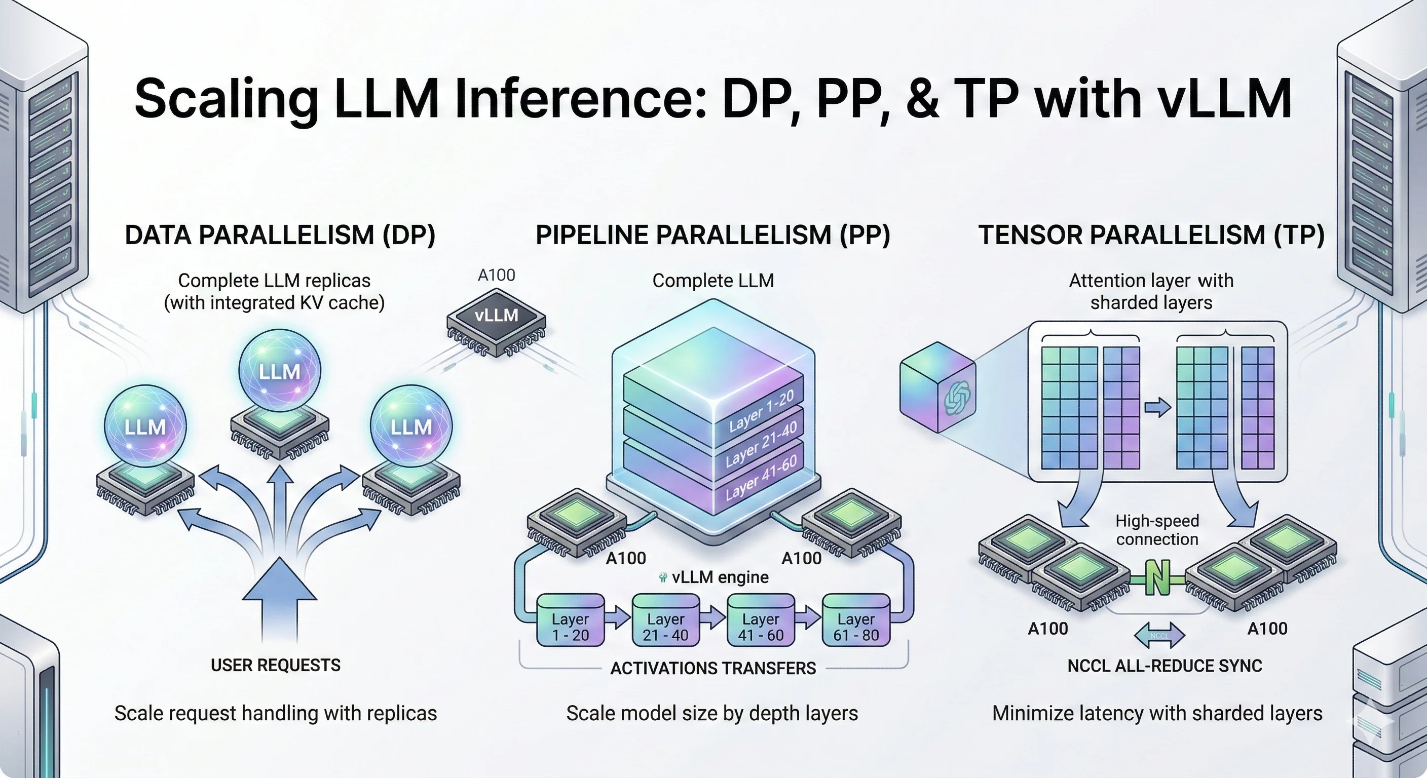
In distributed LLM inference, there are a few core strategies for splitting a model across GPUs like Data Parallelism (DP), Pipeline Parallelism (PP), Tensor Parallelism (TP), Expert Parallelism (EP). In the previous blog, we covered DP, PP, and TP in depth — how they work, when to use them, and how they perform on real models.
In this post, we're focusing on Expert Parallelism (EP) and Mixed strategies like PP+DP, PP+TP. We'll look at why it exists, how it works under the hood in vLLM, and what the numbers look like in practice on a real MoE model and dense models.
Let's begin with Expert Parallelism.
1) Expert Parallelism (EP)
Experts and MoE Models
In a standard transformer, each layer has a large feed-forward network (FFN) basically two big linear layers with an activation in between. Every token passes through the same FFN, so the full weight matrix is always in use.
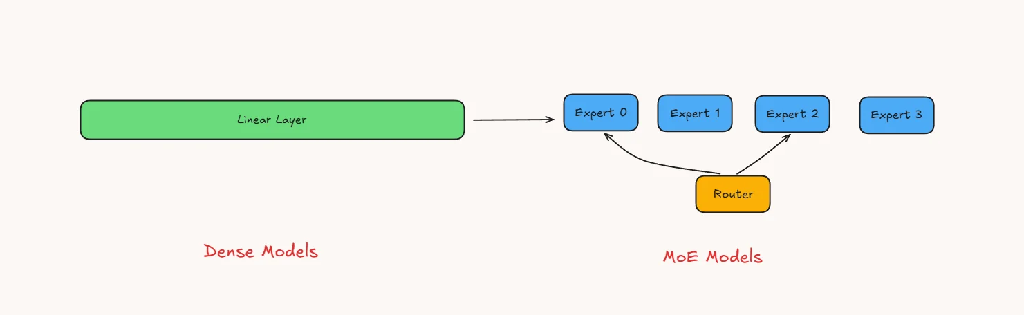
A Mixture-of-Experts (MoE) model takes that single FFN and splits it into several smaller, independent copies called experts. Each expert is its own mini FFN with the same shape but separate weights. A small router (also called a gating network) sits in front of the experts. For every token, the router scores the available experts and selects the top-k experts, where k depends on the model design. In the benchmarked Qwen3.5-35B-A3B model, 8 routed experts plus 1 shared expert are activated per token. Only those selected experts run; the rest stay idle for that token.
This design lets you scale total parameters without scaling compute per token. The model is large in capacity but cheap to run because only a fraction of experts fire each time.
How Experts Are Trained
In a normal transformer, the single big FFN sees every token during training. Gradients flow through the full weight matrix on every step, so all parameters get updated consistently.
With MoE, only the selected experts (say top-2 out of 64) receive gradients for a given token. The remaining experts get zero gradient for that token their weights don't change. Over many batches, each expert gradually specializes based on the tokens the router sends its way.
The router itself is also trained end-to-end. It learns gating scores through the same backpropagation pass, so the routing decisions improve alongside the experts. In practice, an auxiliary load-balancing loss is added to stop the router from always picking the same few experts. Without it, popular experts would keep getting stronger while others starve a problem called expert collapse.
The net effect: MoE training uses roughly the same FLOPs per token as a much smaller dense model, but the total parameter count (and model capacity) is far larger.
Why Expert Parallelism
So we have this MoE model with dozens or hundreds of experts. During inference only a couple of them fire per token, which keeps compute cheap. But here is the problem all those expert weights still need to sit in memory, ready to be picked at any moment.
Take a concrete example. Say a model has 64 experts, each one being a small FFN of about 500 MB. That is 32 GB just for the experts, on top of attention layers, embeddings, and KV cache. A single 80 GB GPU fills up fast. With 128 experts you simply cannot fit the model on one card.
You might think: "just use Tensor Parallelism and split everything across GPUs." Tensor parallelism works well for dense layers, but MoE introduces sparse, token-dependent expert routing. Expert parallelism better matches that structure by colocating expert weights and expert compute, instead of treating the expert block like a uniformly dense layer.
Expert Parallelism takes a smarter approach instead of slicing each expert into pieces, it assigns whole experts to different GPUs. GPU 0 owns experts 0–15, GPU 1 owns experts 16–31, and so on. Each GPU keeps full copies of the shared layers (attention, norms) but only stores its own set of experts. When a token needs expert 20, it gets sent to GPU 1, processed there, and the result comes back. This way memory is balanced, and each GPU only computes what it actually owns.
The tradeoff is communication. Tokens need to travel to wherever their chosen experts live (an all-to-all shuffle), and results need to travel back. On fast interconnects like NVLink this is manageable. On slower PCIe links it can become a bottleneck, especially at high batch sizes where lots of tokens are flying around.
In short, EP exists because MoE models are too big for one GPU but too sparse for naive sharding. It matches the structure of the model independent experts go to independent GPUs.
vLLM Implementation :
The diagram below is a simplified conceptual view of EP with TP=1. When EP is combined with tensor parallelism, the non-expert layers are also partitioned across TP ranks rather than fully replicated on every GPU.
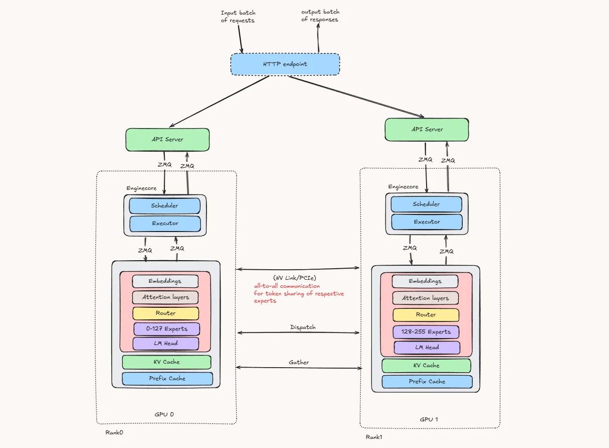
When vLLM runs a MoE model with Expert Parallelism, here is what happens step by step in MoE Layers:
-
The HTTP endpoint receives a batch of incoming requests and sends them to the available API servers.
-
Each API server communicates with its local engine core, which contains the scheduler and executor.
-
On every GPU, the shared parts of the model remain available, including:
- Embeddings
- Attention layers
- LM Head
- KV Cache
- Prefix Cache
-
The experts are divided across GPUs instead of being fully copied on every GPU. As one simple example, experts can be placed contiguously across GPUs. vLLM also supports other expert placement strategies, such as round-robin placement, depending on the deployment configuration.
- GPU 0 stores experts 0–127
- GPU 1 stores experts 128–255
-
Token flow inside the MoE layer
- Token enters the MoE layer: After attention, each token’s hidden state reaches the MoE block.
- Router picks experts: A small gating network scores all experts and selects the top-k experts for that token.
- Tokens are dispatched across GPUs: Since experts are distributed across GPUs, vLLM uses an all-to-all communication step to send each token to the GPU that owns its selected expert.
- Each GPU runs its local experts: Every GPU computes only the expert FFN for the experts it owns, using the tokens it received.
- Results come back: The expert outputs are sent back to the originating GPU, weighted by the router scores, and combined before moving to the next transformer layer.
The main overhead in Expert Parallelism is the all-to-all token shuffle. once when tokens are dispatched to expert-owning GPUs and again when outputs are gathered back. Fast interconnects such as NVLink or InfiniBand help reduce this communication cost.
Experiments (Qwen/Qwen3.5-35B-A3B + ShareGPT)
Getting the Hardware
To run the experiments in this blog post you can rent a GPU at JarvisLabs. Here's how to set up your own instance:
- Log in: JarvisLabs and navigate to the dashboard.
- Create an instance: click Create and select your desired GPU configuration.
- Select your GPU: choose H100 80GB to match the hardware used in this article.
- Choose the framework: select PyTorch from the available frameworks.
- Launch: click Launch. Your instance will be ready in a few minutes.
We ran the experiments in this article on 4× NVIDIA H100 80GB GPUs. If you want to reproduce the reported numbers closely, use the same hardware. Other GPUs may still work for exploratory runs, but the results will differ.
Qwen3.5-35B-A3B is a multimodal model with a vision encoder. For text-only serving, the official vLLM recipe uses --reasoning-parser qwen3 --language-model-only to skip the vision encoder and free additional memory for KV cache.
First, download the ShareGPT dataset:
wget https://huggingface.co/datasets/anon8231489123/ShareGPT_Vicuna_unfiltered/resolve/main/ShareGPT_V3_unfiltered_cleaned_split.jsonBenchmark Command Template
For benchmarking we have tested the same model and prompts with different combination of Expert parallelism with Tensor Parallelism, Data Parallelism and Expert parallelism load balancing techniques. following are the vllm serve and vllm bench commands we have used in this activity.
MoE model without EP with TP
vllm serve Qwen/Qwen3.5-35B-A3B \
   --tensor-parallel-size 2 \
   --gpu-memory-utilization 0.9 \
   --max-model-len 32768
MoE model with EP + TP=2
vllm serve Qwen/Qwen3.5-35B-A3B \
  --tensor-parallel-size 2 \
  --enable-expert-parallel \
  --gpu-memory-utilization 0.9 \
  --max-model-len 32768
MoE model with EP + TP=4
vllm serve Qwen/Qwen3.5-35B-A3B \
  --tensor-parallel-size 4 \
  --enable-expert-parallel \
  --gpu-memory-utilization 0.9 \
  --max-model-len 32768
MoE model with EP + DP=2
vllm serve Qwen/Qwen3.5-35B-A3B \
  --tensor-parallel-size 1 \
  --data-parallel-size 2 \
  --enable-expert-parallel \
  --gpu-memory-utilization 0.9 \
  --max-model-len 32768
MoE model with EP + DP=4
vllm serve Qwen/Qwen3.5-35B-A3B \
  --tensor-parallel-size 1 \
  --data-parallel-size 4 \
  --enable-expert-parallel \
  --gpu-memory-utilization 0.9 \
  --max-model-len 32768
MoE model with EP + DP + EPLB
vllm serve Qwen/Qwen3.5-35B-A3B \
  --tensor-parallel-size 1 \
  --data-parallel-size 2 \
  --enable-expert-parallel \
  --enable-eplb \
  --eplb-config '{"window_size":1000,"step_interval":3000,"log_balancedness":true,"log_balancedness_interval":1}' \
  --gpu-memory-utilization 0.9 \
  --max-model-len 32768
Then run the benchmark:
vllm bench serve \
	--model Qwen/Qwen3.5-35B-A3B \
	--dataset-name sharegpt \
	--dataset-path ./ShareGPT_V3_unfiltered_cleaned_split.json \
	--host 127.0.0.1 \
	--port 8000 \
	--max-concurrency 60 \
	--num-prompts 1000 \
	--seed 42
Concurrency sweep: 60, 120, 180, 240, 300, 360, 420.
Results
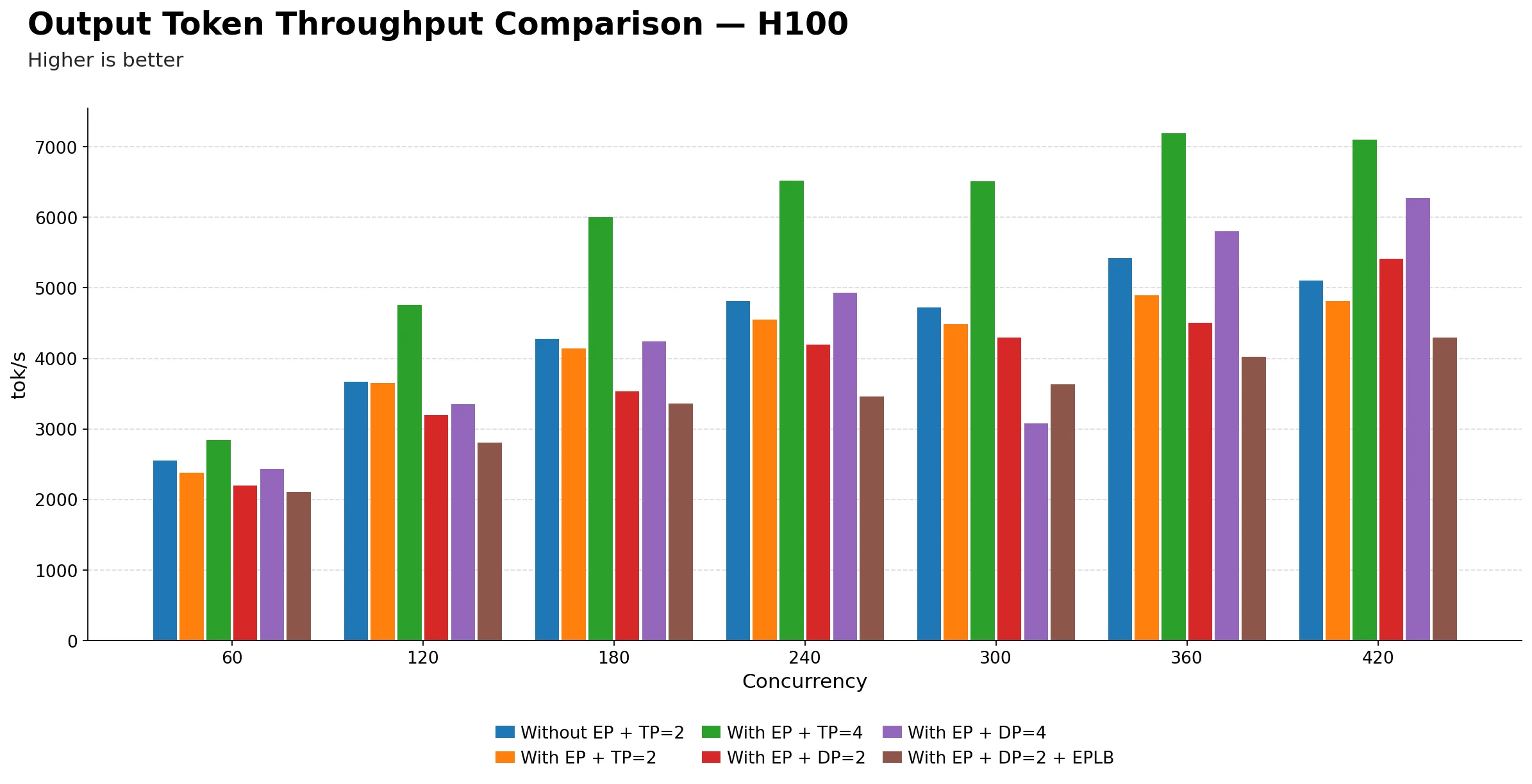
Output token throughput comparison (tok/s)
| Technique | 60 | 120 | 180 | 240 | 300 | 360 | 420 |
|---|---|---|---|---|---|---|---|
| Without EP + TP=2 | 2551.87 | 3667.08 | 4274.36 | 4814.95 | 4725.82 | 5419.30 | 5101.65 |
| With EP + TP=2 | 2383.21 | 3654.54 | 4141.32 | 4548.19 | 4485.26 | 4897.19 | 4812.06 |
| With EP + TP=4 | 2839.85 | 4761.43 | 5999.48 | 6523.35 | 6510.86 | 7188.00 | 7098.50 |
| With EP + DP=2 | 2195.10 | 3192.60 | 3529.91 | 4192.30 | 4296.66 | 4503.15 | 5410.64 |
| With EP + DP=4 | 2429.34 | 3353.99 | 4240.69 | 4927.87 | 3076.26 | 5805.79 | 6276.45 |
| With EP + DP=2 + EPLB | 2108.59 | 2801.63 | 3364.11 | 3455.67 | 3629.08 | 4027.38 | 4291.55 |
-
EP + TP=4 is the clear winner on H100. It leads at every concurrency level from 120 onwards, reaching a peak of 7188.00 tok/s at 360 roughly 33% higher than the baseline Without EP + TP=2 at the same point.
-
At 60 concurrency, Without EP + TP=2 leads among the 2-GPU configs. It reaches 2551.87 tok/s, beating EP + TP=2 (2383.21) and EP + DP=2 (2195.10). EP + TP=4 edges ahead at 2839.85 but uses twice the GPUs, so that comparison isn't apples-to-apples.
-
EP + TP=2 consistently underperforms the baseline Without EP + TP=2. At every single concurrency point, adding EP on top of TP=2 results in lower output throughput. The gap narrows at 120 but never flips, suggesting EP routing overhead is not being offset by any batching benefit at TP=2 scale on H100.
-
EP + DP=4 shows an anomaly at 300. It drops sharply to 3076.26 tok/s far below its neighbors at 240 (4927.87) and 360 (5805.79). This appears to be a significant outlier at that concurrency point. The benchmark table alone shows inconsistent behavior; identifying the exact cause would require profiler traces or engine logs.
-
EP + DP=2 + EPLB is the weakest variant throughout. It is consistently the lowest or near-lowest across all concurrency levels, suggesting that for H100 with this model, EPLB is adding overhead without meaningfully improving expert utilization.
-
EP + DP=4 scales well at high concurrency. From 360 onwards it reaches 6276.45 tok/s at 420, second only to EP + TP=4. So with 4 data-parallel replicas, throughput does scale but the instability at 300 is a concern for production deployments.
-
The key practical takeaway: if you have 4 H100s, EP + TP=4 is the best throughput configuration. If you only have 2, the baseline Without EP + TP=2 is more reliable than adding EP on top of it. EP + DP variants are viable at high concurrency but carry instability risk at certain load points.
Note : We also tried EP + DP=4 + EPLB combination, but it was failing due to some internal bug in vLLM so we skipped it.
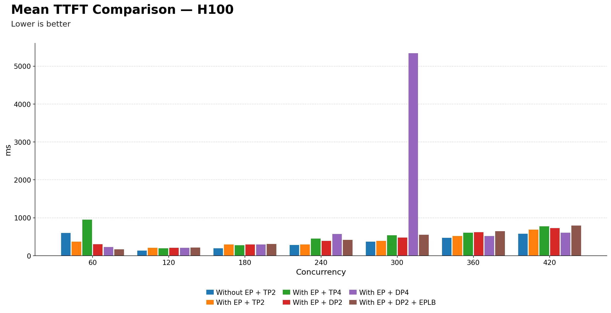
Mean TTFT (ms) comparison
| Technique | 60 | 120 | 180 | 240 | 300 | 360 | 420 |
|---|---|---|---|---|---|---|---|
| Without EP + TP2 | 598.03 | 134.59 | 196.44 | 281.43 | 370.23 | 469.22 | 577.99 |
| With EP + TP2 | 372.44 | 206.34 | 297.98 | 296.38 | 392.42 | 518.78 | 689.87 |
| With EP + TP4 | 953.36 | 193.40 | 276.58 | 453.84 | 536.75 | 607.21 | 776.12 |
| With EP + DP2 | 303.46 | 209.84 | 294.80 | 391.46 | 477.49 | 622.58 | 728.12 |
| With EP + DP4 | 227.92 | 206.94 | 297.16 | 572.58 | 5338.96 | 519.68 | 610.06 |
| With EP + DP2 + EPLB | 165.25 | 212.71 | 312.69 | 417.90 | 552.63 | 650.19 | 795.18 |
-
EP + DP=2 + EPLB delivers the best TTFT at low concurrency. At 60, it reaches just 165.25 ms, significantly better than Without EP + TP=2 (598.03 ms) and EP + TP=4 (953.36 ms). This is a striking reversal from the throughput story the configuration that was weakest on throughput is strongest on first-token latency at low load.
-
EP + TP=4 has surprisingly poor TTFT at 60. At 953.36 ms, it is the worst among all techniques at low concurrency. Despite winning on throughput, the larger TP group may introduce more synchronization overhead during prefill, which is consistent with higher first-token latency when the system is lightly loaded.
-
From 120 to 240, all techniques converge into a relatively tight band. TTFT ranges roughly from 134 ms to 572 ms across all configurations, meaning in moderate-load conditions the choice of parallelism strategy matters less for first-token experience.
-
Without EP + TP=2 degrades sharply after 240. It climbs from 281.43 ms at 240 to 577.99 ms at 420, a steady and notable rise. This is consistent with the baseline configuration running into scheduling pressure as concurrency grows.
-
EP + DP=4 has a severe anomaly at 300. TTFT spikes to 5338.96 ms, completely out of line with its neighbors at 240 (572.58 ms) and 360 (519.68 ms). This is the same configuration that showed a throughput anomaly at 300, suggesting something specific happens at that load point. The tables alone cannot identify the exact cause; profiler traces or engine logs would be needed.
-
EP + TP=4 has the most consistent TTFT growth pattern. It rises steadily from 953 ms at 60 down to 193 ms at 120, then climbs gradually to 776 ms at 420. The dip at 120 before rising again is typical of TP systems that amortize prefill cost better once batches are larger.
-
EPLB does not help TTFT on H100. EP + DP=2 + EPLB is consistently above EP + DP=2 from 120 onwards, meaning enabling load balancing is actually adding latency for first-token delivery in this setup. The benefit only showed at 60, which is not a practically meaningful operating point for a production system.
-
The key practical takeaway: for latency-sensitive workloads at moderate to high concurrency, EP + DP=2 offers the most stable TTFT on H100. EP + TP=4 is a reasonable second choice given its consistency, but its high TTFT at low concurrency makes it a poor fit if the system frequently operates below 120 concurrent requests.
Mean TPOT (ms) comparison
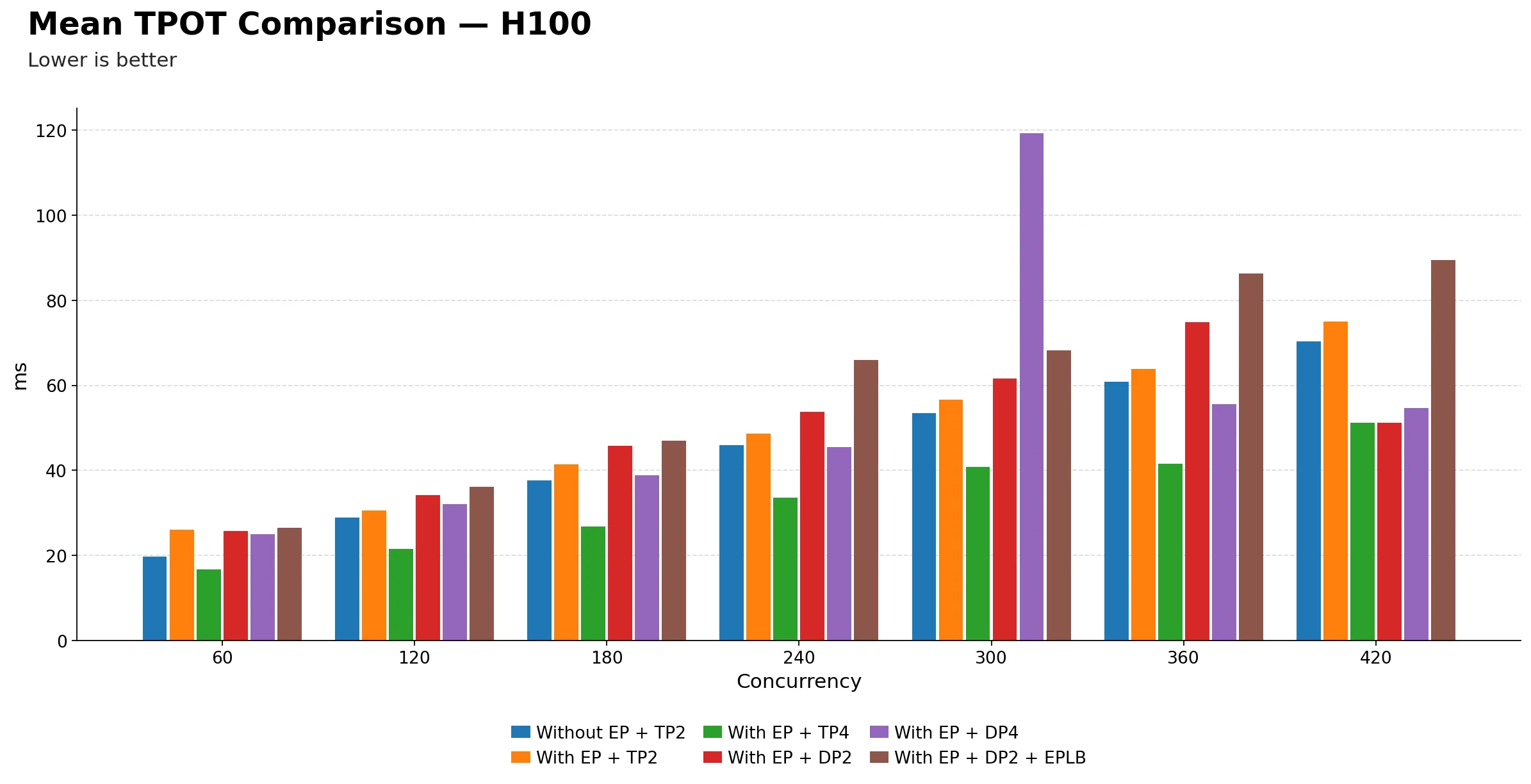
| Technique | 60 | 120 | 180 | 240 | 300 | 360 | 420 |
|---|---|---|---|---|---|---|---|
| Without EP + TP2 | 19.79 | 28.95 | 37.71 | 45.94 | 53.48 | 60.85 | 70.33 |
| With EP + TP2 | 26.12 | 30.51 | 41.38 | 48.64 | 56.69 | 63.83 | 75.00 |
| With EP + TP4 | 16.71 | 21.51 | 26.79 | 33.57 | 40.86 | 41.49 | 51.14 |
| With EP + DP2 | 25.75 | 34.23 | 45.80 | 53.77 | 61.61 | 74.88 | 51.14 |
| With EP + DP4 | 25.07 | 32.09 | 38.78 | 45.51 | 119.21 | 55.59 | 54.62 |
| With EP + DP2 + EPLB | 26.52 | 36.15 | 46.95 | 65.96 | 68.23 | 86.31 | 89.40 |
-
EP + TP=4 dominates TPOT across the entire concurrency range. It starts at 16.71 ms at 60 and only reaches 51.14 ms at 420, staying well below every other technique at every single point. This is the most consistent and clear-cut advantage in the entire benchmark. If decode speed matters, EP + TP=4 is the configuration to use on H100.
-
Without EP + TP=2 and EP + TP=2 are very close throughout. From 60 to 420, they track each other within a few milliseconds. This means adding EP on top of TP=2 neither helps nor hurts per-token decode latency meaningfully, as the overhead and benefit are roughly canceling out.
-
EP + DP=2 + EPLB is consistently the worst configuration for TPOT. It starts at 26.52 ms at 60 and climbs to 89.40 ms at 420, the highest value in the table at every concurrency point from 180 onwards. This is a clear signal that EPLB is adding decode overhead rather than reducing it on H100.
-
EP + DP=4 shows an extreme anomaly at 300. TPOT spikes to 119.21 ms, completely disconnected from its neighbors at 240 (45.51 ms) and 360 (55.59 ms). This is the third metric where EP + DP=4 shows a breakdown at exactly 300 concurrency: throughput dropped, TTFT spiked, and now TPOT does the same. This is consistent with a systemic instability at that operating point.
-
EP + DP=2 has a surprisingly low TPOT at 420. It drops to 51.14 ms, matching EP + TP=4 exactly and well below EP + DP=2 + EPLB (89.40 ms). This looks like an outlier rather than a genuine improvement, and may reflect a measurement artifact or favorable batch composition at that concurrency level.
-
The DP-based variants generally show higher and less stable TPOT than TP-based ones. From 180 onwards, EP + DP=2 and EP + DP=2 + EPLB both climb noticeably faster than the TP-based techniques, confirming that data parallelism with expert routing introduces more decode-time variability under load.
-
TPOT scales more gracefully with TP than DP on H100. The TP-based techniques, both with and without EP, show a smooth, predictable rise in TPOT as concurrency increases. The DP-based variants are choppier and steeper, which is harder to reason about in production.
-
The key practical takeaway: EP + TP=4 is the clear winner for decode latency on H100. For teams where per-token generation speed is a priority, such as streaming or interactive applications, this is the configuration to choose. EP + DP variants trade off decode quality for potential throughput gains, but even that tradeoff is unstable at certain load points like 300 concurrency.
Mean ITL (ms) comparison
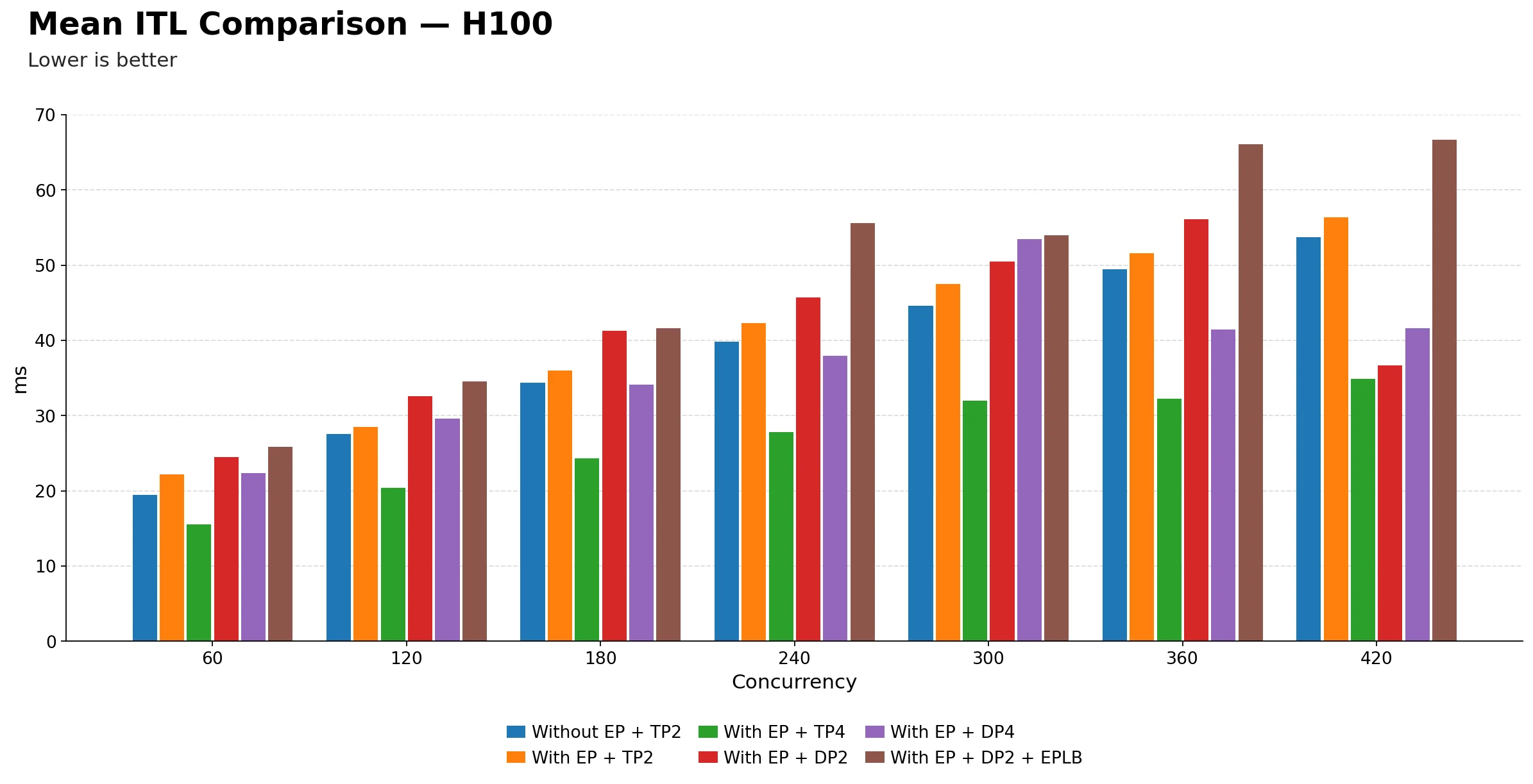
| Technique | 60 | 120 | 180 | 240 | 300 | 360 | 420 |
|---|---|---|---|---|---|---|---|
| Without EP + TP2 | 19.43 | 27.55 | 34.37 | 39.82 | 44.64 | 49.50 | 53.73 |
| With EP + TP2 | 22.15 | 28.51 | 36.03 | 42.29 | 47.52 | 51.60 | 56.36 |
| With EP + TP4 | 15.53 | 20.43 | 24.31 | 27.82 | 31.95 | 32.23 | 34.85 |
| With EP + DP2 | 24.50 | 32.61 | 41.26 | 45.72 | 50.46 | 56.15 | 36.71 |
| With EP + DP4 | 22.34 | 29.64 | 34.13 | 37.96 | 53.48 | 41.47 | 41.58 |
| With EP + DP2 + EPLB | 25.83 | 34.54 | 41.65 | 55.64 | 54.00 | 66.06 | 66.69 |
-
EP + TP=4 again dominates across the entire concurrency range. It starts at 15.53 ms at 60 and only reaches 34.85 ms at 420, maintaining the lowest inter-token latency at every single concurrency point. The gap versus other techniques widens as load increases, making it the most compelling choice for latency-sensitive streaming workloads.
-
Without EP + TP=2 and EP + TP=2 remain very close throughout. Just like TPOT, they track each other within a few milliseconds across the full range. Adding EP on top of TP=2 does not meaningfully change the inter-token experience for end users, suggesting the EP routing overhead and any decode-side benefit are roughly in balance at this scale.
-
EP + DP=2 + EPLB is consistently the worst for ITL. It begins at 25.83 ms at 60, already the highest in the table, and climbs to 66.69 ms at 420. At every concurrency point from 60 onwards it sits above all other techniques, reinforcing the pattern seen in TPOT that EPLB is adding latency overhead rather than reducing it on H100.
-
EP + DP=4 shows the same breakdown at 300. ITL spikes to 53.48 ms, significantly above its neighbors at 240 (37.96 ms) and 360 (41.47 ms). This is now the fourth metric covering throughput, TTFT, TPOT, and ITL, where EP + DP=4 shows a clear anomaly at exactly 300 concurrency. This is a consistent pattern suggesting instability at that operating point; however, confirming the root cause would require profiler traces or engine logs.
-
EP + DP=2 shows an unexpectedly low ITL at 420. It drops to 36.71 ms, well below EP + DP=2 + EPLB (66.69 ms) and even below the baseline Without EP + TP=2 (53.73 ms). Similar to the TPOT observation, this looks like an outlier rather than a reliable improvement, possibly reflecting favorable batch composition or a scheduling artifact at that specific load point.
-
The gap between TP-based and DP-based techniques grows steadily with concurrency. At 60 the difference is small, roughly 6 to 10 ms, but by 420 the TP-based techniques are around 35 to 56 ms while DP-based variants sit at 37 to 67 ms. The separation is modest in absolute terms but consistent in direction, confirming that TP handles decode-time token pacing better under load.
-
ITL scales more smoothly with TP than DP on H100. The TP-based curves rise gradually and predictably. The DP-based curves are choppier, with EP + DP=4 in particular showing sharp swings. For production systems where consistent token delivery matters, such as real-time streaming, this unpredictability is a meaningful concern.
-
The key practical takeaway: EP + TP=4 is the best configuration for inter-token latency on H100. It delivers roughly half the ITL of the DP-based variants at high concurrency, with no anomalies across the full range. For any application where smooth, responsive token streaming is a priority, this is the clear recommendation.
2) Mixing Parallelism Strategies on 4 GPUs
In the previous blog post we looked at each parallelism strategy on its own Tensor Parallelism, Pipeline Parallelism, and Data Parallelism one at a time. But in practice you often have multiple GPUs and need to combine strategies to get the best balance of throughput and latency.
In this section we take 4 GPUs and try two different combinations:
- Pipeline Parallelism(PP) + Data Parallelism(DP) : split the model into 2 pipeline stages, then run 2 data-parallel replicas. This gives you two independent copies of the model, each spread across 2 GPUs by layers. Good for handling more requests at the same time.
- Pipeline Parallelism(PP) + Tensor Parallelism : split the model into 2 pipeline stages, and within each stage use tensor parallelism across 2 GPUs. This keeps a single replica but makes each stage faster by distributing the matrix math. Good for lower per-request latency.
We use Qwen/Qwen3-32B as our test model. It is a 32-billion parameter dense model, large enough and a good fit for seeing how different parallelism mixes behave.
For benchmarking we use 1000 prompts from the ShareGPT dataset with a fixed seed, sweeping concurrency from 60 to 660 to see how each setup handles increasing load.
A) Pipeline Parallelism(PP) + Data Parallelism(DP)
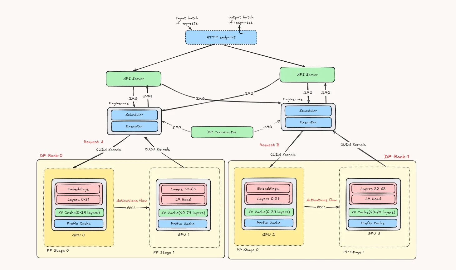
This diagram shows how pipeline parallelism (PP) and data parallelism (DP) work together in vLLM.
At the top, incoming requests first reach the HTTP endpoint, which then forwards them to the available API servers. These API servers are connected to multiple EngineCore processes through ZMQ. Each EngineCore is responsible for one data parallel rank.
In this example, we have DP Rank 0 and DP Rank 1. You can think of these as two separate replicas of the same model setup. The main reason for DP is to let the system handle more requests at the same time. So one request can go to DP Rank 0 while another goes to DP Rank 1.
Inside each DP rank, the model is split using pipeline parallelism. Instead of putting the full model on one GPU, the layers are divided across two GPUs:
- PP Stage 0 holds the embeddings and the first half of the transformer layers
- PP Stage 1 holds the second half of the layers and the LM head
So if Request A is assigned to DP Rank 0, it first runs on GPU 0, where the early layers are computed. The intermediate activations are then sent to GPU 1, which finishes the remaining layers and produces the output. The same thing happens on the other side for Request B inside DP Rank 1, using GPU 2 and GPU 3.
Each pipeline stage also keeps the KV cache for the layers it owns. That means the cache is naturally split stage by stage, instead of one GPU storing everything. The prefix cache is also local to that rank, which helps reuse repeated prompt prefixes.
The DP Coordinator sits in the control plane and talks to the EngineCores. Its role is not to run model layers, but to help coordinate the data-parallel engines.
A simple way to read the picture is:
DP creates multiple copies of the serving stack, and PP splits each copy across GPUs by layers.
So in practice:
- DP helps with throughput
- PP helps fit and run larger models across multiple GPUs
- and together they let vLLM serve more requests while still spreading one model replica across stages
B) Pipeline Parallelism(PP) + Tensor Parallelism
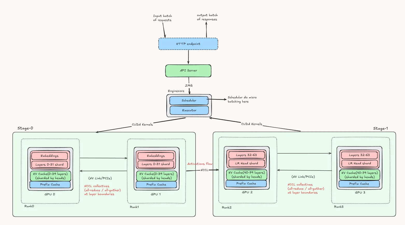 This diagram shows how pipeline parallelism (PP) and tensor parallelism (TP) are combined in vLLM to split one model across multiple GPUs.
The request first reaches the HTTP endpoint, then the API server, and from there it is passed to the EngineCore. Inside the EngineCore, the scheduler handles batching and decides how requests are executed, while the executor coordinates the GPU workers.
In this example, the model is divided into two pipeline stages. Stage 0 contains the embeddings and the first half of the transformer layers, while Stage 1 contains the remaining layers and the LM head. This is the pipeline parallel part: the model is split by layer ranges, and the request moves forward stage by stage.
At the same time, each stage is also split across two GPUs using tensor parallelism. That means the layers inside a stage are not stored as one full block on a single GPU. Instead, the computation for those layers is shared across the two GPUs in that stage. So Stage 0 is handled jointly by one TP group, and Stage 1 is handled jointly by another TP group.
When a request arrives, it first runs through Stage 0, where both GPUs in that stage cooperate to process the embeddings and early layers. Once that part is done, the resulting hidden states are passed to Stage 1. There again, both GPUs in the second stage work together to process the later layers and produce the final logits.
So the key idea is simple: PP splits the model across stages, and TP splits each stage across multiple GPUs. Because of that, a single request moves through the pipeline stage by stage, while the GPUs inside each stage work together on every layer in that stage.
This setup is useful when the model is too large or too heavy for a single GPU. Pipeline parallelism helps divide the model into manageable chunks, and tensor parallelism helps distribute the computation of each chunk across multiple GPUs. Together, they allow vLLM to run larger models efficiently while still keeping all GPUs actively involved in the forward pass.
Benchmarks :
vLLM commands :
For PP + DP :
CUDA_VISIBLE_DEVICES=0,1,2,3 \
vllm serve Qwen/Qwen3-32B \
  --dtype bfloat16 \
  --pipeline-parallel-size 2 \
  --data-parallel-size 2 \
  --gpu-memory-utilization 0.90
For PP + TP :
CUDA_VISIBLE_DEVICES=0,1,2,3 \
vllm serve Qwen/Qwen3-32B \
  --dtype bfloat16 \
  --pipeline-parallel-size 2 \
  --tensor-parallel-size 2 \
  --gpu-memory-utilization 0.90
Because DP creates multiple serving ranks, we also checked that batching and scheduler-related limits were configured consistently across runs so the PP + DP and PP + TP comparison remained meaningful.
Output Token Throughput (tok/s)
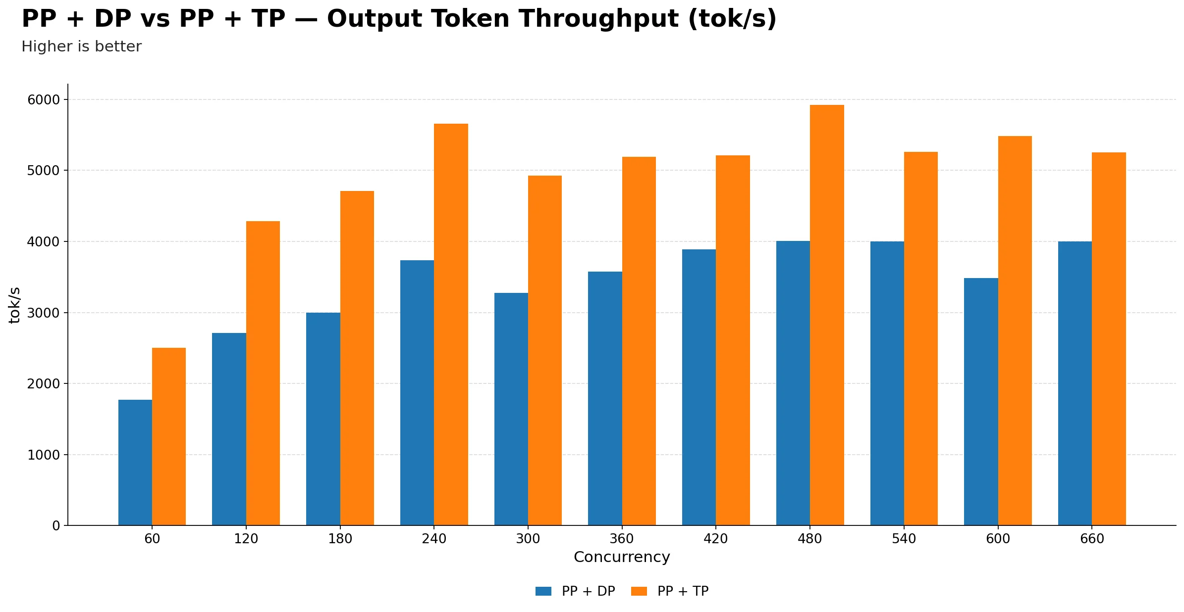
| Metric | 60 | 120 | 180 | 240 | 300 | 360 | 420 | 480 | 540 | 600 | 660 |
|---|---|---|---|---|---|---|---|---|---|---|---|
| PP + DP | 1773.68 | 2713.45 | 2993.42 | 3736.61 | 3276.84 | 3574.06 | 3887.58 | 4008.34 | 4000.68 | 3484.90 | 3997.93 |
| PP + TP | 2499.10 | 4288.90 | 4712.26 | 5661.00 | 4928.99 | 5191.30 | 5210.46 | 5922.35 | 5257.96 | 5485.96 | 5250.91 |
-
PP + TP delivers significantly higher throughput than PP + DP across the entire concurrency range. At peak, PP + TP reaches about 5922 tok/s at 480 while PP + DP peaks at about 4008.34 tok/s at 480, roughly a ~47.8% advantage for PP + TP. If raw output throughput is the primary goal, PP + TP is the clear winner.
-
Both configurations peak around 480 concurrency. After that point, neither gains meaningfully from additional requests. This suggests the saturation point is driven by the pipeline depth and model size rather than the parallelism strategy, and pushing beyond 480 hurts latency without reward in either case.
-
PP + DP shows less smooth scaling than PP + TP. PP + DP has noticeable throughput dips at 300 and 600, whereas PP + TP rises more consistently through its operating range. This suggests PP + DP is more susceptible to batching inefficiencies and pipeline bubbles as load fluctuates.
-
At low concurrency, the gap between the two is already large. At 60, PP + TP produces about 2500 tok/s versus 1774 tok/s for PP + DP. So even when the system is lightly loaded, PP + TP makes better use of available compute, likely because tensor parallelism reduces per-layer latency more effectively than pipeline stages.
-
Beyond 480, extra concurrency mostly hurts latency without giving meaningful throughput gains for either configuration. PP + TP plateaus in the 5.2k–5.9k tok/s band while PP + DP hovers around 3.5k–4.0k tok/s. The throughput advantage of PP + TP is persistent and does not narrow at high load.
Mean TTFT (ms)
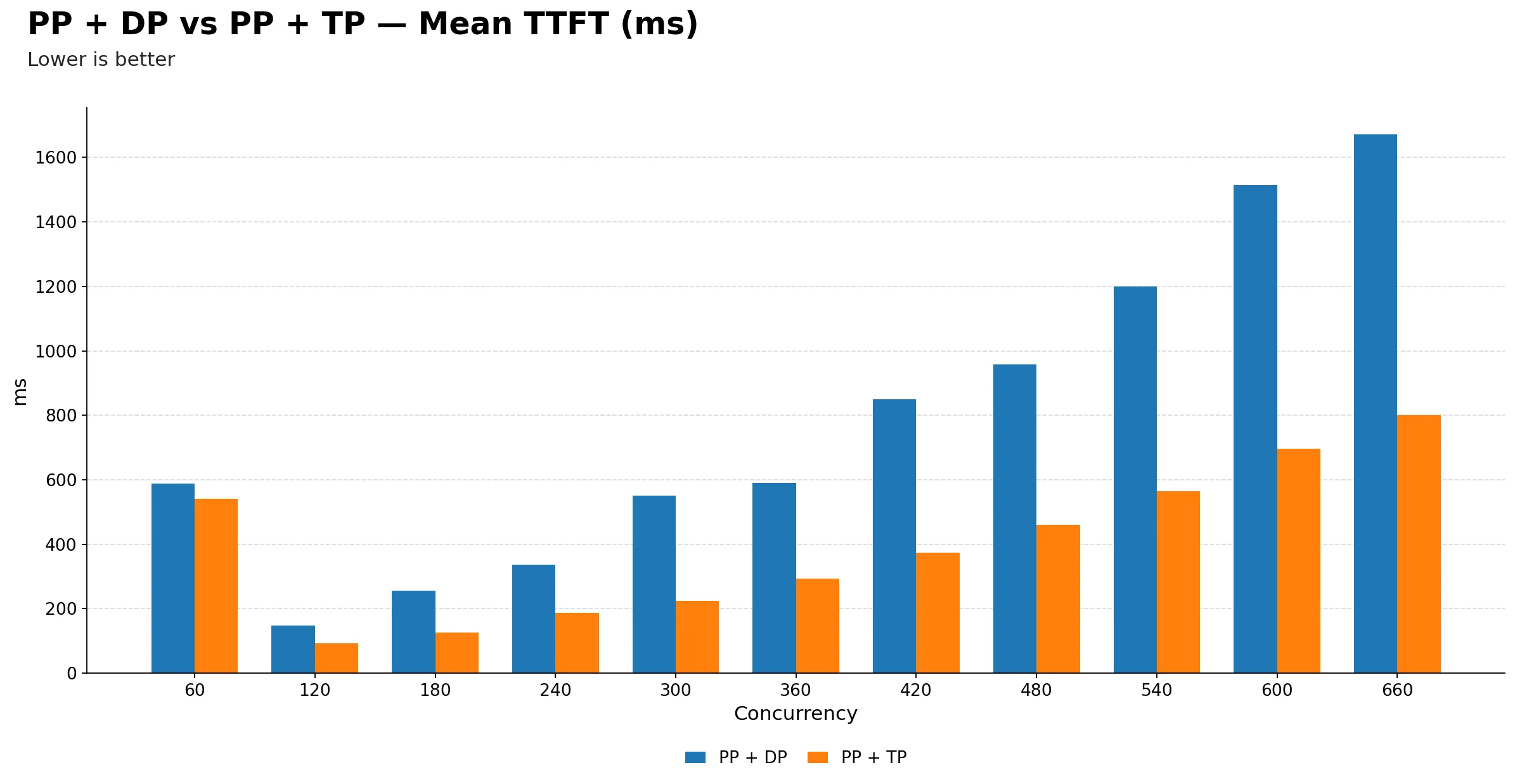
| Metric | 60 | 120 | 180 | 240 | 300 | 360 | 420 | 480 | 540 | 600 | 660 |
|---|---|---|---|---|---|---|---|---|---|---|---|
| PP + DP | 588.86 | 147.92 | 255.82 | 336.79 | 550.58 | 589.53 | 849.15 | 957.19 | 1198.74 | 1513.43 | 1671.33 |
| PP + TP | 541.75 | 93.23 | 125.23 | 186.72 | 225.02 | 293.12 | 373.38 | 460.40 | 564.72 | 696.65 | 799.71 |
-
PP + TP is consistently better on TTFT across the full concurrency range. The gap starts modest at 60, roughly 580 ms vs 540 ms, but widens dramatically at higher concurrency, reaching about 1660 ms for PP + DP versus 800 ms for PP + TP at 660. So PP + TP is more than twice as responsive for first-token delivery under heavy load.
-
Both configurations share the same inflection at 120. TTFT drops sharply from 60 to 120 for both, then climbs steadily. This is a consistent signal that both setups are underutilized at the lowest concurrency and only start batching efficiently once enough requests arrive.
-
PP + DP TTFT degrades much more steeply after 300. From 300 onwards the blue bars grow rapidly: 550 ms, 590 ms, 850 ms, 960 ms, 1200 ms, 1510 ms, 1660 ms, while PP + TP climbs much more gradually through 225 ms, 295 ms, 375 ms, 460 ms, 560 ms, 695 ms, 800 ms. This suggests pipeline stage synchronization in PP + DP may become a bottleneck under heavy prefill pressure.
-
For latency-sensitive workloads, PP + TP is the safer choice at any concurrency above 180. The TTFT gap becomes too large to ignore from that point onwards, and only keeps growing.
Mean TPOT (ms)
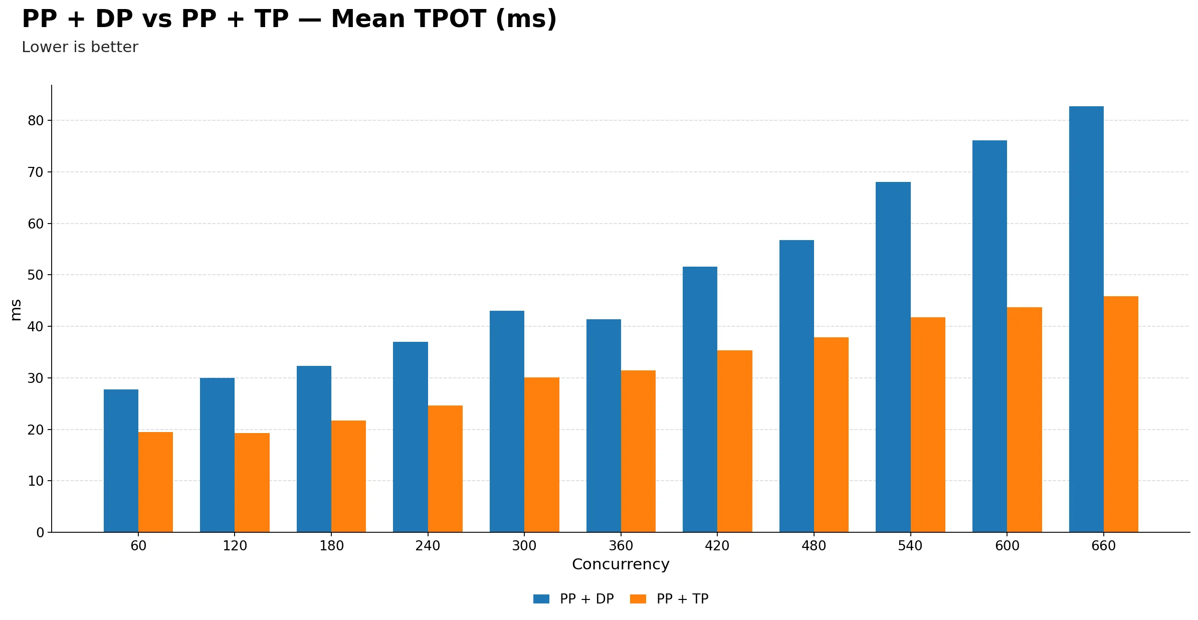
| Metric | 60 | 120 | 180 | 240 | 300 | 360 | 420 | 480 | 540 | 600 | 660 |
|---|---|---|---|---|---|---|---|---|---|---|---|
| PP + DP | 27.78 | 29.98 | 32.32 | 36.97 | 43.00 | 41.33 | 51.55 | 56.74 | 68.01 | 76.14 | 82.72 |
| PP + TP | 19.52 | 19.31 | 21.74 | 24.62 | 30.11 | 31.40 | 35.33 | 37.91 | 41.73 | 43.68 | 45.85 |
-
PP + TP has consistently lower TPOT throughout. It starts around 19.5 ms at 60 and only reaches 45.9 ms at 660, while PP + DP starts at 27.8 ms and climbs all the way to 82.7 ms. At peak concurrency, PP + DP users are waiting nearly twice as long per generated token compared to PP + TP.
-
The gap is already visible at 60 and only widens with load. Even at the lowest concurrency, PP + TP has a roughly 8 ms TPOT advantage. This early gap suggests the structural overhead of pipeline parallelism hurts decode efficiency even when the system is lightly loaded.
-
PP + DP TPOT accelerates sharply after 420. It jumps from about 51 ms at 420 to 68 ms at 540 and then 83 ms at 660, a steep climb in the high-concurrency region. PP + TP by contrast stays relatively flat from 420 onwards, rising only from 35 ms to 46 ms in the same range.
-
For any application where token generation speed matters, whether streaming, interactive use, or real-time responses, PP + TP is the clear choice. The TPOT advantage is consistent, growing, and not sensitive to the operating concurrency point.
Mean ITL (ms)
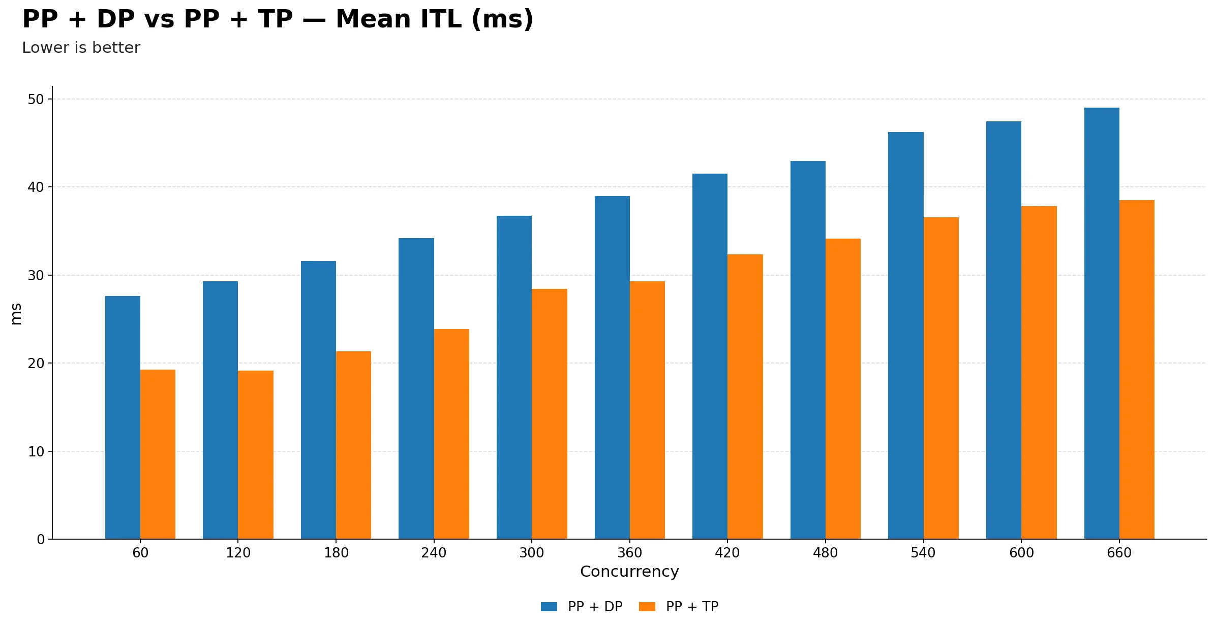
| Metric | 60 | 120 | 180 | 240 | 300 | 360 | 420 | 480 | 540 | 600 | 660 |
|---|---|---|---|---|---|---|---|---|---|---|---|
| PP + DP | 27.61 | 29.31 | 31.59 | 34.21 | 36.73 | 38.96 | 41.54 | 42.94 | 46.26 | 47.42 | ~49.00 |
| PP + TP | 19.27 | 19.12 | 21.34 | 23.88 | 28.45 | 29.29 | 32.36 | 34.14 | 36.57 | 37.84 | 38.49 |
-
PP + TP maintains lower inter-token latency at every single concurrency point. The orange bars are consistently shorter than the blue bars across the full range, with no crossover. This is the most visually clean result in the entire comparison. PP + TP simply wins on ITL everywhere.
-
The gap starts at roughly 8 ms at low concurrency and grows to about 11 ms at 660. While the absolute difference is not enormous, it is persistent and directionally consistent. For streaming applications where users perceive token pacing, even a few milliseconds per token adds up noticeably over a long response.
-
PP + DP ITL climbs steadily without plateauing. It goes from 27.5 ms at 60 to ~49.00 ms at 660, a near doubling. PP + TP also rises but more gradually, from 19.3 ms to 38.5 ms. The slower growth in PP + TP suggests tensor parallelism handles decode-side scheduling pressure more gracefully than pipeline stages.
-
The key practical takeaway: PP + TP is the better choice in every dimension examined. It delivers higher throughput, lower TTFT, better TPOT, and more stable ITL. PP + DP only makes sense if tensor parallelism is not feasible due to model architecture constraints or GPU interconnect limitations, where pipeline parallelism becomes the only viable multi-GPU strategy.
Verdict
PP + TP is the superior strategy across every metric tested. There is no concurrency point in the entire benchmark where PP + DP wins on throughput, TTFT, TPOT, or ITL. The advantage is not marginal. At high concurrency, PP + TP delivers roughly ~47.8% more output tokens per second, 2x better first-token latency, and nearly half the per-token decode time. This is a consistent and decisive result, not a close call.
The only scenario where PP + DP would be a reasonable choice is when the model architecture or GPU interconnect topology makes tensor parallelism impractical, for example when GPUs are not connected via NVLink and all-reduce communication over slower interconnects would negate the TP benefit. In that constrained case, PP + DP becomes a fallback rather than a preference.
The Expert Parallelism experiments on Qwen3.5-35B-A3B on H100 tell the same story from a different angle. EP + TP=4 is the standout configuration, peaking at 7188 tok/s at 360 concurrency, roughly 33% above the no-EP baseline, while simultaneously delivering the lowest TPOT (16 to 51 ms) and ITL (15 to 35 ms) across the entire sweep. Adding EP on top of TP=2 yields no meaningful throughput gain over the baseline and no perceptible improvement in decode latency. DP-based EP configurations scale more erratically, with EP + DP=4 collapsing at exactly 300 concurrency across every metric. EPLB adds routing overhead without improving expert utilization on H100, making it a net negative for production use with this model.
Conclusion
Across both experiment sets, the direction is consistent. PP + TP outperforms PP + DP on every metric for dense models, and EP + TP=4 is the standout configuration for MoE models. The practical operating sweet spot for the mixed-parallelism dense-model experiments is 240 to 480 concurrency, where throughput is near its peak and latency has not yet degraded severely.
If you have 4 GPUs with fast interconnects, PP + TP should be your default serving configuration for dense models of this size, and EP + TP=4 is the equivalent choice for MoE models. Reserve DP-based configurations for situations where NVLink or equivalent high-bandwidth GPU-to-GPU connectivity is unavailable and tensor parallelism communication costs become prohibitive.
What's Next
Choosing the right GPU matters as much as choosing the right parallelism strategy — see our H100 vs A100 comparison for benchmarks on the hardware used in this post.
In the next post we are diving deep into Context Parallelism (CP), the strategy for scaling inference across very long sequences.
We will walk through how the prompt is split across GPUs during prefill, why queries stay local while keys and values are gathered globally, and how token generation works once the KV cache is distributed. We will also run a full benchmark covering throughput, TTFT, TPOT, and ITL across different sequence lengths and concurrency levels, so you have concrete numbers to guide your own deployments.
Stay tuned.
Get Started
Build & Deploy Your AI in Minutes
Cloud GPU infrastructure designed specifically for AI development. Start training and deploying models today.
View Pricing